High Collinearity Effect in Regressions

Giuliano Sposito included in data science

2018-01-19 1490 words 7 minutes

/2018-01-19-high-collinearity-effect-in-regressions/images/surface_cost.jpg

Contents

Collinearity refers to the situation in which two or more predictor variables collinearity are closely related to one another. The presence of collinearity can pose problems in the regression context, since it can be difficult to separate out the individual effects of collinear variables on the response.

This R Notebook seeks to ilustrate some of the difficulties that can be result from a collinearity.

Collinearity

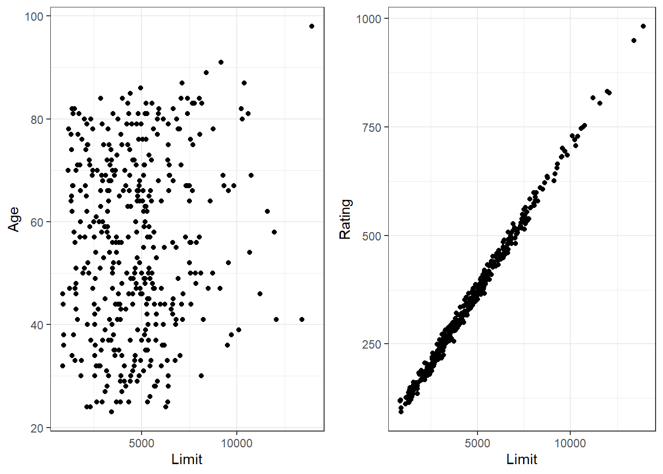
The concept of collinearity is illustrated in Figure below using the Credit data set in the ISLR Package. In the left-hand panel of Figure the two predictors limit and age appear to have no obvious relationship. In contrast, in the right-hand panel the predictors limit and rating are very highly correlated with each other, and we say that they are collinear.¹

 1
 2
 3
 4
 5
 6
 7
 8
 9
10
11
12
13
14
15
16
17
18
19


# setup
library(ISLR)
library(tidyverse)
library(ggplot2)
library(grid)
library(gridExtra)

# ploting Limit by Age
ggplot(Credit, aes(x=Limit, y=Age)) +
  geom_point() +
  theme_bw() -> p1

# ploting Limit by Rating
ggplot(Credit, aes(x=Limit, y=Rating)) +
  geom_point() +
  theme_bw() -> p2

# Ploting side-by-side
marrangeGrob(list(p1,p2), nrow=1, ncol=2, top=NULL)

Effect on a Model

Let’s fit two models using these pair of features (age x limit and Rating x Limit) to predict the Balance outcome and see what happen with the model performances

1
2
3


# balance in function of Age and Limit
fit_axl <- lm(Balance~Age+Limit, Credit)
summary(fit_axl)

 1
 2
 3
 4
 5
 6
 7
 8
 9
10
11
12
13
14
15
16
17
18
19


## 
## Call:
## lm(formula = Balance ~ Age + Limit, data = Credit)
## 
## Residuals:
##     Min      1Q  Median      3Q     Max 
## -696.84 -150.78  -13.01  126.68  755.56 
## 
## Coefficients:
##               Estimate Std. Error t value Pr(>|t|)    
## (Intercept) -1.734e+02  4.383e+01  -3.957 9.01e-05 ***
## Age         -2.291e+00  6.725e-01  -3.407 0.000723 ***
## Limit        1.734e-01  5.026e-03  34.496  < 2e-16 ***
## ---
## Signif. codes:  0 '***' 0.001 '**' 0.01 '*' 0.05 '.' 0.1 ' ' 1
## 
## Residual standard error: 230.5 on 397 degrees of freedom
## Multiple R-squared:  0.7498,	Adjusted R-squared:  0.7486 
## F-statistic:   595 on 2 and 397 DF,  p-value: < 2.2e-16

The first is a regression of balance on age and limit, here both age and limit are highly significant with very small p-values.

1
2
3


# balance in function of Rating and Limit
fit_rxl <- lm(Balance~Rating+Limit, Credit)
summary(fit_rxl)

 1
 2
 3
 4
 5
 6
 7
 8
 9
10
11
12
13
14
15
16
17
18
19


## 
## Call:
## lm(formula = Balance ~ Rating + Limit, data = Credit)
## 
## Residuals:
##    Min     1Q Median     3Q    Max 
## -707.8 -135.9   -9.5  124.0  817.6 
## 
## Coefficients:
##               Estimate Std. Error t value Pr(>|t|)    
## (Intercept) -377.53680   45.25418  -8.343 1.21e-15 ***
## Rating         2.20167    0.95229   2.312   0.0213 *  
## Limit          0.02451    0.06383   0.384   0.7012    
## ---
## Signif. codes:  0 '***' 0.001 '**' 0.01 '*' 0.05 '.' 0.1 ' ' 1
## 
## Residual standard error: 232.3 on 397 degrees of freedom
## Multiple R-squared:  0.7459,	Adjusted R-squared:  0.7447 
## F-statistic: 582.8 on 2 and 397 DF,  p-value: < 2.2e-16

In the second, the collinearity between limit and rating has caused the standard error for the limit coefficient estimate to increase by a factor of 12 and the p-value to increase to 0.701. In other words, the importance of the limit variable has been masked due to the presence of collinearity.

Collinearity reduces the accuracy of the estimates of the regression coefficients, it causes the standard error for $ \hat{ \beta } _{j} $ to grow. Recall that the t-statistic for each predictor is calculated by dividing $ \hat{ \beta } _{j} $ by its standard error. Consequently, collinearity results in a decline in the t-statistic. As a result, in the presence of collinearity, we may fail to reject $ H0 : \beta _{j} = 0 $ . This means that the power of the hypothesis test-the probability of correctly power detecting a non-zero coefficient-is reduced by collinearity.

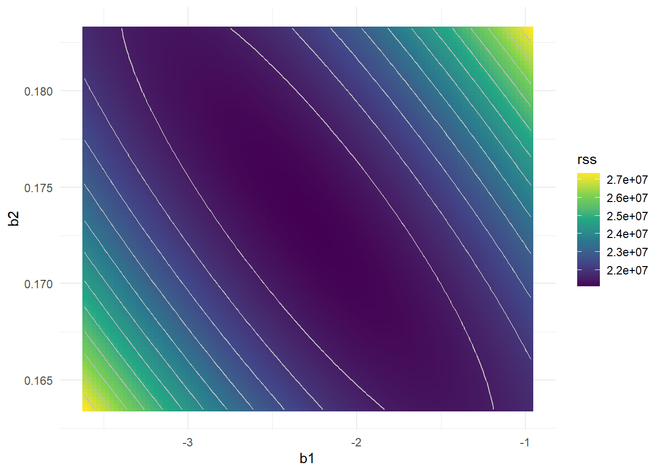
Cost Surface

Why the collinearity reduces the accuracy of the regression coefficients? What is the effect of it in the fitting model? To visualize the effect lets plot the Cost Function surface (RSS) in the space of the coefficents.

Age x Limit

 1
 2
 3
 4
 5
 6
 7
 8
 9
10
11
12
13
14
15
16
17
18
19
20
21
22
23
24
25
26
27
28
29
30
31
32
33
34
35
36
37
38
39
40
41
42
43
44


# generate variations of parameters around 95% interval
# to build the parameters variation scenario.
getConfInterval95 <- function(model, res){
  intercept <- coef(model)[1]
  cfit <- confint(model)
  b1_range <- seq(cfit[2,1], cfit[2,2], abs((cfit[2,1]-cfit[2,2])/res))
  b2_range <- seq(cfit[3,1], cfit[3,2], abs((cfit[3,1]-cfit[3,2])/res))
  expand.grid(int=intercept,
              b1=b1_range,
              b2=b2_range)
}


# calc RSS from target and prediction
rss <- function(y,y_hat){
  sum((y - y_hat)^2)
}

# apply X to Theta parameters and calc the RSS from a target Y
calcRSS <- function(X,Th,Y){
  Y_hat <- cbind(1,X) %*% t(Th)
  rss(Y,Y_hat)
}

# get range variations for the parameters in the Age x Limit model
axl_var <- getConfInterval95(fit_axl, 100)

# calc the RSS for each parameter variation
axl_var$rss <- apply(
  axl_var,
  1,
  function(th){
    calcRSS( X = as.matrix(Credit[,c("Age","Limit")]),
              Th = t(th),
              Y = as.matrix(Credit[,"Balance"]) )
  }
)

axl_var %>% 
  ggplot(aes(x=b1, y=b2, z=rss, fill=rss)) +
  geom_raster() +
  geom_contour(color="grey") +
  scale_fill_viridis_c() +
  theme_minimal()

Rating x Limit

 1
 2
 3
 4
 5
 6
 7
 8
 9
10
11
12
13
14
15
16
17
18
19
20


# get range variations for the parameters in the Rating x Limit model
rxl_var <- getConfInterval95(fit_rxl, 100)

# calc the RSS for each parameter variation
rxl_var$rss <- apply(
  rxl_var,
  1,
  function(th){
    calcRSS( X = as.matrix(Credit[,c("Rating","Limit")]),
              Th = t(th),
              Y = as.matrix(Credit[,"Balance"]) )
  }
)

rxl_var %>% 
  ggplot(aes(x=b1, y=b2, z=rss, fill=rss)) +
  geom_raster() +
  geom_contour(color="grey") +
  scale_fill_viridis_c() +
  theme_minimal()

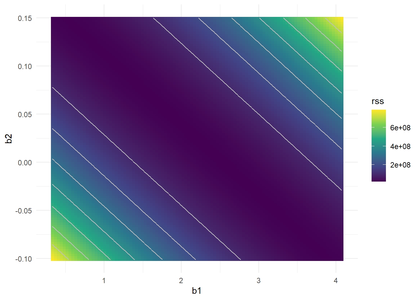
Interestingly, even though the limit and rating coefficients now have much more individual uncertainty, they will almost certainly lie somewhere in this contour valley. For example, we would not expect the true value of the limit and rating coefficients to be ???0.1 and 1 respectively, even though such a value is plausible for each coefficient individually.

Correlation Matrix

A simple way to detect collinearity is to look at the correlation matrix of the predictors. An element of this matrix that is large in absolute value indicates a pair of highly correlated variables, and therefore a collinearity problem in the data. Unfortunately, not all collinearity problems can be detected by inspection of the correlation matrix: it is possible for collinearity to exist between three or more variables even if no pair of variables has a particularly high correlation. We call this situation multicollinearity.²

 1
 2
 3
 4
 5
 6
 7
 8
 9
10
11
12
13
14


# calc the correlation between the features
Credit %>%
  select(-ID, -Balance) %>% # remove "ID" and "Target" Column
  mutate_if(is.factor, as.numeric) %>% # converting factors to num
  as.matrix() -> creditMatrix 
  
# we can computhe the correlation matrix fom 'cor' function
corCredMtx <- cor(creditMatrix)

# rendering
corCredMtx %>% 
  round(2) %>% 
  knitr::kable() %>% 
  kableExtra::kable_styling(font_size = 9)

	Income	Limit	Rating	Cards	Age	Education	Gender	Student	Married	Ethnicity
Income	1.00	0.79	0.79	-0.02	0.18	-0.03	-0.01	0.02	0.04	-0.03
Limit	0.79	1.00	1.00	0.01	0.10	-0.02	0.01	-0.01	0.03	-0.02
Rating	0.79	1.00	1.00	0.05	0.10	-0.03	0.01	0.00	0.04	-0.02
Cards	-0.02	0.01	0.05	1.00	0.04	-0.05	-0.02	-0.03	-0.01	0.00
Age	0.18	0.10	0.10	0.04	1.00	0.00	0.00	-0.03	-0.07	-0.03
Education	-0.03	-0.02	-0.03	-0.05	0.00	1.00	-0.01	0.07	0.05	-0.03
Gender	-0.01	0.01	0.01	-0.02	0.00	-0.01	1.00	0.06	0.01	0.00
Student	0.02	-0.01	0.00	-0.03	-0.03	0.07	0.06	1.00	-0.08	-0.03
Married	0.04	0.03	0.04	-0.01	-0.07	0.05	0.01	-0.08	1.00	0.06
Ethnicity	-0.03	-0.02	-0.02	0.00	-0.03	-0.03	0.00	-0.03	0.06	1.00

1
2
3
4


# the corrPlot package has a good way to plot a correlation matrix
library(corrplot)
corrplot(corCredMtx, type = "upper", order = "hclust", 
         tl.col = "black", tl.srt = 45)

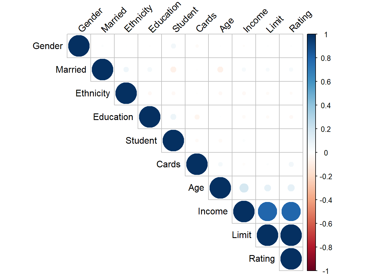
We see in the chart that income, limit and rating are highly correlated between, what is expected in term of finalcial credit.

Conclusion

When faced with the problem of collinearity, there are two simple solutions. The first is to drop one of the problematic variables from the regression. This can usually be done without much compromise to the regression fit, since the presence of collinearity implies that the information that this variable provides about the response is redundant in the presence of the other variables.

The second solution is to combine the collinear variables together into a single predictor. For instance, we might take the average of standardized versions of limit and rating in order to create a new variable that measures credit worthiness.

References

Gareth James, Daniela Witten, Trevor Hastie, Robert Tibshirani. Introduction to Statistical Learning in R, p.99 ↩︎
Gareth James, Daniela Witten, Trevor Hastie, Robert Tibshirani. Introduction to Statistical Learning in R, p.101 ↩︎