Putting your workout to move

Giuliano Sposito included in data science

2018-01-20 585 words 3 minutes

/2018-01-20-putting-your-workout-to-move/images/cover.jpg

Contents

In this quick post, we’ll take one MTB ride, tracked by FitBit in a TXC File, and generate a animated gif. Using gganimate Package and using the same code we learned, we can animate the map with few words.

Reading TCX File

We already saw to how read and GPS track information stored in a TXC/GPX file, once it’s just an XML File.

 1
 2
 3
 4
 5
 6
 7
 8
 9
10
11
12
13
14
15
16
17
18
19
20
21
22
23
24
25
26
27
28
29
30
31
32
33
34
35


library(XML)
library(lubridate)
library(tidyverse)
library(ggmap)
library(gganimate)
library(knitr)

file <- "data/11654237848.tcx"

pfile <- htmlTreeParse(file = file,
                       error = function (...) {},
                       useInternalNodes = TRUE)

features <- c("time", "position/latitudedegrees", "position/longitudedegrees",
              "altitudemeters", "distancemeters", "heartratebpm/value")

fnames <- c("dt", "lat", "lon", "alt", "dist", "hbpm")

"//trackpoint/" %>%
  paste0(features) %>%
  map(function(p){xpathSApply(pfile, path = p, xmlValue)}) %>%
  setNames(fnames) %>%
  as_data_frame() %>% 
  mutate_at(vars(lat:dist), as.numeric) %>%
  mutate(
    dt = lubridate::as_datetime(dt),
    hbpm  = as.integer(hbpm),
    tm.prev.s = c(0, diff(dt)),
    tm.cum.min  = round(cumsum(tm.prev.s)/60,1)
  ) -> track

track %>% 
  head(10) %>% 
  kable() %>% 
  kableExtra::kable_styling(font_size = 9)

dt	lat	lon	alt	dist	hbpm	tm.prev.s	tm.cum.min
2018-01-06 10:34:08	-22.70375	-46.75608	683.59	0.00	111	0	0.0
2018-01-06 10:34:12	-22.70375	-46.75608	683.59	0.02	111	4	0.1
2018-01-06 10:34:13	-22.70375	-46.75608	683.30	0.05	111	1	0.1
2018-01-06 10:34:14	-22.70375	-46.75609	683.59	0.11	111	1	0.1
2018-01-06 10:34:15	-22.70374	-46.75610	684.09	0.79	111	1	0.1
2018-01-06 10:34:16	-22.70373	-46.75611	684.09	2.37	111	1	0.1
2018-01-06 10:34:17	-22.70372	-46.75611	684.59	4.08	111	1	0.1
2018-01-06 10:34:18	-22.70371	-46.75609	685.20	5.94	110	1	0.2
2018-01-06 10:34:19	-22.70369	-46.75608	685.50	7.83	110	1	0.2
2018-01-06 10:34:20	-22.70367	-46.75607	685.10	9.80	110	1	0.2

Plot the map

Also we saw how is easy to plot the track over a map using ggmap package.

 1
 2
 3
 4
 5
 6
 7
 8
 9
10
11


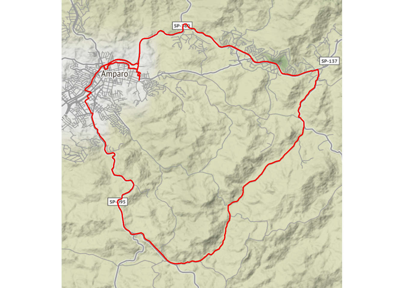
# getting the map backgroubd 
bbox <- make_bbox(lon = track$lon, lat=track$lat, f=.1)
gmap <- get_map( location=bbox, maptype = "terrain", source="google")

# base plot
ggmap(gmap) + 
  geom_path(data=track, mapping=aes(lon, lat),
            color="red", alpha = 1, size = 0.8, lineend = "round") +
  coord_fixed() +
  theme_void() +
  theme( legend.position = "none" )

Animating the Map

Now, with a little more code, we can use the gganimate Package to create a animated gif version of this plot.

gganimate plotting a series of ggplots and put them together in a gif (or other format) using ImageMagick. Two aesthetics keywords in the ggplot2 grammar are in charge to control how the individual charts will be gerated: frame and cumulative. The first indicate which feature in the data frame is the “time dimention” and the other controls if the plot will be incremental (from a “frame” to “frame”) or cumulative (from “beginning” to the “current frame”).

 1
 2
 3
 4
 5
 6
 7
 8
 9
10
11
12
13
14
15
16
17
18
19
20
21


# lets make a frame each 3 minutes
# to not destroy the track info, we collapse the data on each 3 minutes
track %>%
  mutate(
    dt = floor_date(dt, "3 minutes")
  ) -> track

# base plot
ggmap(gmap) + 
  # cumulative layer, the "whole path" along the time (dt)
  geom_path(data=track, mapping=aes(lon, lat, frame=dt, cumulative=T),
            color="yellow", alpha = 1, size = 0.8, lineend = "round") +
  # the "instant" plot, the 3 minutes path in the frame (dt)
  geom_path(data=track, mapping=aes(lon, lat, frame=dt, cumulative=F),
            size=1.2, lineend = "round", color="red") +
  coord_fixed() +
  theme_void() +
  theme( legend.position = "none" ) -> p

p <- gganimate(p, interval=0.01, ani.width=400,
               ani.height=400, filename = "11654237848.gif" )