Ploting your MTB track with R

Giuliano Sposito included in data science

2018-01-16 1655 words 8 minutes

/2018-01-16-ploting-your-mtb-track-with-r/images/mtb_cover.jpg

Contents

In this RNotebook we’ll read a TCX and GPX files, used to track physical training and exercises evolving GPS and paths used by some workout Mobile Apps and Devices. Particularly we’ll will process one TCX file containing a MTB ride mine and transforming the a useful R data.frame ploting the ride track over a map.

Tracking Files¹

There are two popular file format to track workouts and routes through GPS devices: GPX and TCX.

GPX is an XML format designed specifically for saving GPS track, way point and route data. It is increasingly used by GPS programs because of its flexibility as an XML schema. More information can be found on the official GPX website.

The TCX format is also an XML format, but was created by Garmin to include additional data with each track point (e.g. heart rate and cadence) as well as a user defined organizational structure. The format appears to be primarily used by Garmin’s fitness oriented GPS devices. The TCX schema is hosted by Garmin.

Many of the dozens of other formats can be converted into GPX or TCX formats using GPSBabel.

Reading a TCX File

Lets see what is the basic format of one TCX file, once it’s a XML file we just open it in a text editor to look at. I downloaded one from a MTB ride that I did using a FitBit Charge 2, plus an iPhone as tracker.

 1
 2
 3
 4
 5
 6
 7
 8
 9
10
11
12
13
14
15
16
17
18
19
20
21
22
23
24
25
26
27
28
29
30
31
32
33
34
35
36
37
38
39
40
41
42
43
44
45
46
47
48
49
50



<?xml version="1.0" encoding="UTF-8" standalone="yes"?>
<TrainingCenterDatabase xmlns="http://www.garmin.com/xmlschemas/TrainingCenterDatabase/v2">
    <Activities>
        <Activity Sport="Biking">
            <Id>2018-01-13T08:15:42.000-02:00</Id>
            <Lap StartTime="2018-01-13T08:15:42.000-02:00">
                <TotalTimeSeconds>12672.0</TotalTimeSeconds>
                <DistanceMeters>42274.04000000001</DistanceMeters>
                <Calories>2315</Calories>
                <Intensity>Active</Intensity>
                <TriggerMethod>Manual</TriggerMethod>
                <Track>
                    <Trackpoint>
                        <Time>2018-01-13T08:15:42.000-02:00</Time>
                        <Position>
                            <LatitudeDegrees>-22.703736066818237</LatitudeDegrees>
                            <LongitudeDegrees>-46.75607788562775</LongitudeDegrees>
                        </Position>
                        <AltitudeMeters>684.7</AltitudeMeters>
                        <DistanceMeters>0.0</DistanceMeters>
                        <HeartRateBpm>
                            <Value>104</Value>
                        </HeartRateBpm>
                    </Trackpoint>
                    <Trackpoint>
                        <Time>2018-01-13T08:15:47.000-02:00</Time>
                        <Position>
                            <LatitudeDegrees>-22.703736066818237</LatitudeDegrees>
                            <LongitudeDegrees>-46.75607788562775</LongitudeDegrees>
                        </Position>
                        <AltitudeMeters>684.7</AltitudeMeters>
                        <DistanceMeters>6.240000000000001</DistanceMeters>
                        <HeartRateBpm>
                            <Value>102</Value>
                        </HeartRateBpm>
                    </Trackpoint>
                    
                    ...
                    
            </Lap>
            <Creator xsi:type="Device_t" xmlns:xsi="http://www.w3.org/2001/XMLSchema-instance">
                <Name>Fitbit Charge 2</Name>
                <UnitId>0</UnitId>
                <ProductID>0</ProductID>
            </Creator>
        </Activity>
    </Activities>
</TrainingCenterDatabase>

As we see, it’s a time-date indexed XML file with some structuring to define activities and inside them activity with summary informations, laps and track points.

Let’s extract the available tracking data (date-time, latitude and longitude coords, altitude and heart beat) from this file, using the XML Package. Because with are just interested in the GPS data we can use XPath Query directly to take the track points data through all the XML file.

 1
 2
 3
 4
 5
 6
 7
 8
 9
10
11
12
13
14
15
16
17
18
19
20
21
22
23
24
25
26
27
28
29
30
31
32
33
34
35
36
37
38
39


# setup
library(XML)
library(lubridate)
library(tidyverse)

# Reading the XML file
file <- htmlTreeParse(file = "data/11654237848.tcx", # file downloaded from FitBit
                       error = function (...) {},
                       useInternalNodes = TRUE)

# XML nodes names to read 
features <- c("time", "position/latitudedegrees", "position/longitudedegrees",
              "altitudemeters", "distancemeters", "heartratebpm/value")

# building the XPath query adding the "father node"
xpath_feats <- paste0("//trackpoint/", features)

# for each of the XPaths let's extract the value of the node
xpath_feats %>%
  # the map returns a list with vector of the values for each xpath
  map(function(p){xpathSApply(file, path = p, xmlValue)}) %>%
  # setting a shorter name for them and collapsing the list in to a tibble
  setNames(c("dt", "lat", "lon", "alt", "dist", "hbpm")) %>%
  as_tibble() %>% 
  # Lets correct the data type because everthing return as char
  mutate_at(vars(lat:dist), as.numeric) %>% # numeric values
  mutate(
    dt = lubridate::as_datetime(dt), # date time
    hbpm  = as.integer(hbpm), # integer (heart beat per minutes)
    # we'll build other two features:  
    tm.prev.s = c(0, diff(dt)), # time (s) from previous track point
    tm.cum.min  = round(cumsum(tm.prev.s)/60,1) # cumulative time (min)
  ) -> track

# lets see the final format
track %>% 
  head(10) %>% 
  knitr::kable() %>% 
  kableExtra::kable_styling(font_size = 9)

dt	lat	lon	alt	dist	hbpm	tm.prev.s	tm.cum.min
2018-01-06 10:34:08	-22.70375	-46.75608	683.59	0.00	111	0	0.0
2018-01-06 10:34:12	-22.70375	-46.75608	683.59	0.02	111	4	0.1
2018-01-06 10:34:13	-22.70375	-46.75608	683.30	0.05	111	1	0.1
2018-01-06 10:34:14	-22.70375	-46.75609	683.59	0.11	111	1	0.1
2018-01-06 10:34:15	-22.70374	-46.75610	684.09	0.79	111	1	0.1
2018-01-06 10:34:16	-22.70373	-46.75611	684.09	2.37	111	1	0.1
2018-01-06 10:34:17	-22.70372	-46.75611	684.59	4.08	111	1	0.1
2018-01-06 10:34:18	-22.70371	-46.75609	685.20	5.94	110	1	0.2
2018-01-06 10:34:19	-22.70369	-46.75608	685.50	7.83	110	1	0.2
2018-01-06 10:34:20	-22.70367	-46.75607	685.10	9.80	110	1	0.2

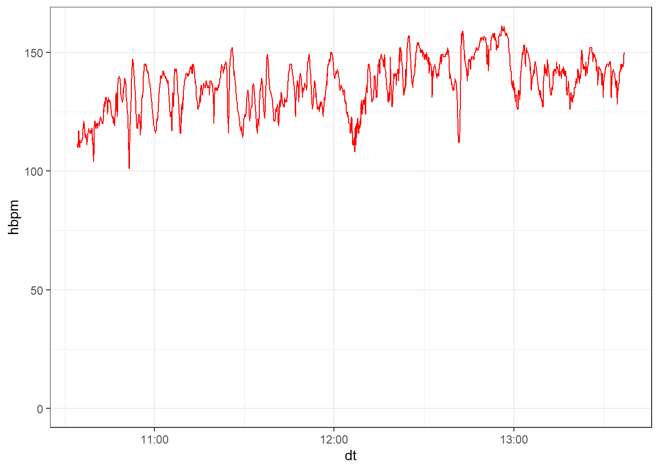
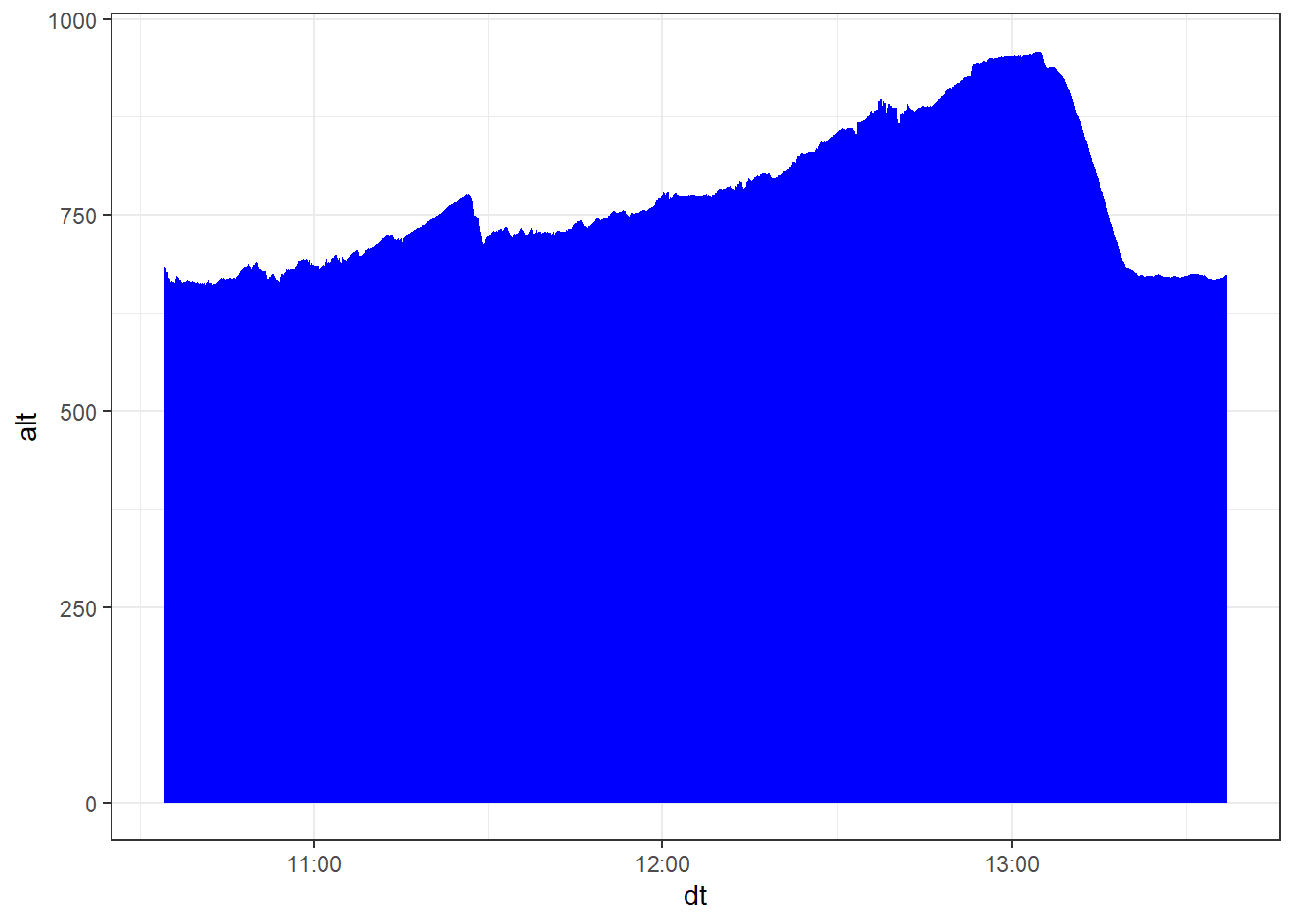
With the data set in hand, we can use the info, for examplar to plot the heart beat and altitude.

1
2
3
4


library(ggplot2)

ggplot(track, aes(x=dt, y=hbpm)) + 
  geom_line(colour="red") + theme_bw() + ylim(0,max(track$hbpm))

1
2
3


ggplot(track) +
  geom_area(aes(x = dt, y = alt), fill="blue", stat="identity") +
  theme_bw() 

Ploting the track

We can take the latitude and longitude coordenates extract from TCX and plot the path executed during this ride. This is pretty straighforward using geom_path()in ggplot2.

1
2
3
4
5
6


# ploting latitude in N/S orietation and lon as E/L orientation
ggplot(track, aes(x=lon, y=lat)) +
  geom_path(aes(colour=alt), size=1.2) + # ploting alt as color reference
  scale_colour_gradientn(colours = terrain.colors(10)) + # color scale
  coord_fixed() + # to keep the aspect ratio
  theme_void() # removint axis

That’s cool, we extract the GPS path from TCX file and plot them with a couple of lines, just remaining plot over a map, and this is easy too, using ggmappackage.

Ploting over a map

The ggmap R Package is a collection of functions to visualize spatial data and models on top of static maps from various online sources (e.g Google Maps and Stamen Maps). It includes tools common to those tasks, including functions for geolocation and routing.

The package uses some providers to get a “background” image to be used as base map, also maps the scale of the image to the appropriate lat/lon coordenates.

 1
 2
 3
 4
 5
 6
 7
 8
 9
10
11
12


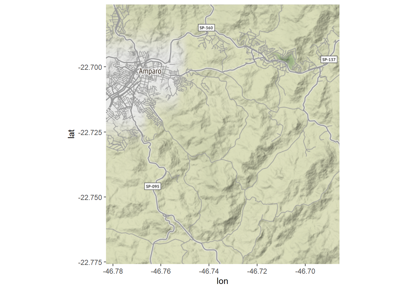
library(ggmap)

# first we define a "box" based on lats and lons that will ploted over
# the make_bbox build it.
bbox <- make_bbox(lon = track$lon, lat=track$lat, f=.1)

# after that we ask for a map containing this box to one of the providers
# in this case we'll ask for google maps a 'terrain map'
gmap <- get_map( location=bbox, maptype = "terrain", source="google")

# we can see the map obtained
ggmap(gmap)

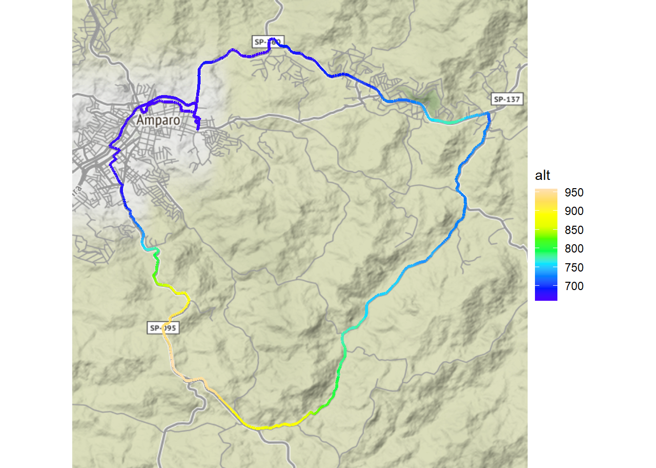
Once with the map background in hands, we just plot the track over it, changing the color scale to improve the contrast.

1
2
3
4
5
6
7


# now the ggmap is the base o ggplot
ggmap(gmap) +
  # ploting the path using lon and lat as coordenates and alt as color
  geom_path(data=track, aes(x=lon, y=lat, colour=alt), size=1.2) + 
  scale_colour_gradientn(colours = topo.colors(10)) + # color scale
  coord_fixed() + # to keep the aspect ratio
  theme_void() # removint axis

Conclusion

As we saw, it’s pretty straightforward to get the data in the XML and transform them in a useful R data frame. Obviously if the XML was more complicated, with several activities and laps, we should handle this info if we want keep these informations before read the trackpoints. The data frame with track points would gain activity.id and lap.id columns. The use of ggmap is very helpful to use maps and gglot together.

Appendix: Reading a GPX file

Basically, as we using XPath to get the data points, reading a GPX file is pretty the same, let’s look the structure of one file exported from Runtastic website

 1
 2
 3
 4
 5
 6
 7
 8
 9
10
11
12
13
14
15
16
17
18
19
20
21
22
23
24
25
26
27
28
29
30
31
32
33
34
35
36
37
38
39



<?xml version="1.0" encoding="UTF-8"?>
<gpx version="1.1" creator="Runtastic: Life is short - live long, http://www.runtastic.com" xsi:schemaLocation="http://www.topografix.com/GPX/1/1
                                http://www.topografix.com/GPX/1/1/gpx.xsd
                                http://www.garmin.com/xmlschemas/GpxExtensions/v3
                                http://www.garmin.com/xmlschemas/GpxExtensionsv3.xsd
                                http://www.garmin.com/xmlschemas/TrackPointExtension/v1
                                http://www.garmin.com/xmlschemas/TrackPointExtensionv1.xsd" xmlns="http://www.topografix.com/GPX/1/1" xmlns:gpxtpx="http://www.garmin.com/xmlschemas/TrackPointExtension/v1" xmlns:gpxx="http://www.garmin.com/xmlschemas/GpxExtensions/v3" xmlns:xsi="http://www.w3.org/2001/XMLSchema-instance">
  <metadata>
    <desc>Ate o Barracao de Itapira. Volta pelo Jardim Vitoria atras do Cristo e Faz. Palmeiras.</desc>
    <copyright author="www.runtastic.com">
      <year>2017</year>
      <license>http://www.runtastic.com</license>
    </copyright>
    <link href="http://www.runtastic.com">
      <text>runtastic</text>
    </link>
    <time>2017-06-11T11:45:00.000Z</time>
  </metadata>
  <trk>
    <link href="http://www.runtastic.com/sport-sessions/1698893337">
      <text>Visit this link to view this activity on runtastic.com</text>
    </link>
    <trkseg>
      <trkpt lon="-46.7560615539550781" lat="-22.7035655975341797">
        <ele>677.462890625</ele>
        <time>2017-06-11T11:45:00.000Z</time>
      </trkpt>
      <trkpt lon="-46.7560310363769531" lat="-22.7035102844238281">
        <ele>677.3987426757812</ele>
        <time>2017-06-11T11:45:02.000Z</time>
      </trkpt>
      
      ...
      
      </trkseg>
  </trk>
</gpx>

Basically it’s about same, with a metadata in the beginning and the track points are in the nodes trkpt, but the struct is different. The GPS coords are attributes of these nodes while elevation and time are sub-nodes in the value. We’ll have to use XPath different to get the value and the attributes.

 1
 2
 3
 4
 5
 6
 7
 8
 9
10
11
12
13
14
15
16
17
18
19
20
21
22
23
24
25
26
27
28
29


# reading the xml file download from runtastic
file <- htmlTreeParse(file = "./data/runtastic_20170611_1134_Cycling.gpx",
                      error = function (...) {},
                      useInternalNodes = TRUE)

# reading the ATTRIBUTES of 'trkpt' nodes
coords <- xpathSApply(file, path = "//trkpt", xmlAttrs) # <- look parameter xmlAttrs
lat <- as.numeric(coords["lat", ])
lon <- as.numeric(coords["lon", ])

# reading node values
ele <- as.numeric(xpathSApply(file, path = "//trkpt/ele", xmlValue)) # <- look parameter xmlValue
dt <- lubridate::as_datetime(xpathSApply(file, path = "//trkpt/time", xmlValue)) # <- look parameter xmlValue

# buiding the data frame
tibble(
  dt = dt,
  lat = lat,
  lon = lon, 
  alt = ele
) %>% mutate(
  tm.prev.s = c(0, diff(dt)), # time (s) from previous track point
  tm.cum.min  = round(cumsum(tm.prev.s)/60,1) # cumulative time (min)
) -> gpx.track

gpx.track %>% 
  head(10) %>% 
  knitr::kable() %>% 
  kableExtra::kable_styling(font_size = 9)

dt	lat	lon	alt	tm.prev.s	tm.cum.min
2017-06-11 11:45:00	-22.70357	-46.75606	677.4629	0	0.0
2017-06-11 11:45:02	-22.70351	-46.75603	677.3987	2	0.0
2017-06-11 11:45:05	-22.70347	-46.75600	677.3459	3	0.1
2017-06-11 11:45:08	-22.70337	-46.75598	677.2225	3	0.1
2017-06-11 11:45:10	-22.70330	-46.75596	677.0735	2	0.2
2017-06-11 11:45:13	-22.70319	-46.75595	676.7396	3	0.2
2017-06-11 11:45:16	-22.70307	-46.75594	676.2781	3	0.3
2017-06-11 11:45:18	-22.70299	-46.75592	675.7316	2	0.3
2017-06-11 11:45:21	-22.70288	-46.75592	675.1077	3	0.3
2017-06-11 11:45:24	-22.70276	-46.75592	674.4054	3	0.4

References

http://www.earlyinnovations.com/gpsphotolinker/about-gpx-and-tcx-file-formats.html ↩︎