Using ggmap and gganimation to visualize oil spill in Brazil coastline

In 2019, a crude oil spill struck more than 2,000 kilometers off the coast of Brazil’s Northeast and Southeast, affecting more than 400 beaches in more than 200 different municipalities. The first reports of the spill occurred at the end of August with sightings still spreading later this year. This post explores the sighting records available on the IBAMA website to view the impact of the leak using ggmap and gganimation.
In 2019, a crude oil spill struck more than 2,000 kilometers off the coast of Brazil’s Northeast and Southeast, affecting more than 400 beaches in more than 200 different municipalities. The first reports of the spill occurred at the end of August with sightings still spreading later this year. More than a thousand tons of oil have already been collected from the beaches, which is the worst oil leak in Brazil’s history and the largest environmental disaster on the Brazilian coastline.
In this post we will explore the oil sighting data, published on the IBAMA website (the Brazilian Institute of the Environment and Renewable Natural Resources), a state agency from the Ministry of the Environment responsible for implementing federal environmental preservation policies. We’ll try to view the oil spill extension and evolution using the ggmap and gganimation R packages.
Site and Dataset
IBAMA has made the oil spill data and information available on a subsection of its site, keeping a daily record of status and spotting sightings.
Part of the records provided are available in excel format, and according with it’s description, the files contain: the name of each spotted location, the county, the date of first sighting, the state, latitude, longitude, date where the location was revisited and oil spill status at the moment.
Data Scrapping
Although the site offers PDF and XLXS, and it is possible to explore the sightings table within PDF files through the tabulizer package, in this post we’ll only explore the contents of the excel files. The first step to this is to scrap the page that provides the files to download, to extract its links, we’ll use rvest package to do this job.
|
|
| date | description | items | type | link |
|---|---|---|---|---|
| 2019-12-14 | Localidades Atingidas | PDF - 32MB | http://www.ibama.gov.br/phocadownload/emergenciasambientais/2019/manchasdeoleo/2019-12-14_LOCALIDADES_AFETADAS.pdf | |
| 2019-12-14 | Localidades Atingidas | XLSX - 74KB | XLSX | http://www.ibama.gov.br/phocadownload/emergenciasambientais/2019/manchasdeoleo/2019-12-14_LOCALIDADES_AFETADAS.xlsx |
| 2019-12-13 | Localidades Atingidas | PDF - 32MB | http://www.ibama.gov.br/phocadownload/emergenciasambientais/2019/manchasdeoleo/2019-12-13_LOCALIDADES-AFETADAS.pdf | |
| 2019-12-13 | Localidades Atingidas | XLSX - 73KB | XLSX | http://www.ibama.gov.br/phocadownload/emergenciasambientais/2019/manchasdeoleo/2019-12-13_LOCALIDADES-AFETADAS_planilha.xlsx |
| 2019-12-12 | Localidades Atingidas | PDF - 31,3MB | http://www.ibama.gov.br/phocadownload/emergenciasambientais/2019/manchasdeoleo/2019-12-12_LOCALIDADES_AFETADAS.pdf | |
| 2019-12-12 | Localidades Atingidas | XLSX - 72.2KB | XLSX | http://www.ibama.gov.br/phocadownload/emergenciasambientais/2019/manchasdeoleo/2019-12-12_LOCALIDADES_AFETADAS.xlsx |
| 2019-12-11 | Localidades Atingidas | PDF - 31.4MB | http://www.ibama.gov.br/phocadownload/emergenciasambientais/2019/manchasdeoleo/2019-12-11_LOCALIDADES_AFETADAS.pdf | |
| 2019-12-11 | Localidades Atingidas | XLSX - 78KB | XLSX | http://www.ibama.gov.br/phocadownload/emergenciasambientais/2019/manchasdeoleo/2019-12-11_LOCALIDADES_AFETADAS_planilha.xlsx |
| 2019-12-10 | Localidades Atingidas | PDF - 31MB | http://www.ibama.gov.br/phocadownload/emergenciasambientais/2019/manchasdeoleo/2019-12-10_LOCALIDADES-AFETADAS.pdf | |
| 2019-12-10 | Localidades Atingidas | XLSX - 68KB | XLSX | http://www.ibama.gov.br/phocadownload/emergenciasambientais/2019/manchasdeoleo/2019-12-10_LOCALIDADES-AFETADAS.xlsx |
Now that we have the links in hand, let’s download the XLSX files.
|
|
| date | description | items | type | link | filename |
|---|---|---|---|---|---|
| 2019-10-16 | Localidades Atingidas | XLSX - 15KB | XLSX | http://www.ibama.gov.br/phocadownload/emergenciasambientais/2019/manchasdeoleo/2019-10-16_LOCALIDADES_AFETADAS.xlsx | ./data/oil_leakage_raw/2019-10-16.xlsx |
| 2019-10-17 | Localidades Atingidas | XLSX - 15KB | XLSX | http://www.ibama.gov.br/phocadownload/emergenciasambientais/2019/manchasdeoleo/2019-10-17_LOCALIDADES_AFETADAS.xlsx | ./data/oil_leakage_raw/2019-10-17.xlsx |
| 2019-10-18 | Localidades Atingidas | XLSX - 15KB | XLSX | http://www.ibama.gov.br/phocadownload/emergenciasambientais/2019/manchasdeoleo/2019-10-18_LOCALIDADES_AFETADAS.xlsx | ./data/oil_leakage_raw/2019-10-18.xlsx |
| 2019-10-19 | Localidades Atingidas | XLSX - 44KB | XLSX | http://www.ibama.gov.br/phocadownload/notas/2019/2019-10-19_LOCALIDADES_AFETADAS_PLANILHA.xls | ./data/oil_leakage_raw/2019-10-19.xlsx |
| 2019-10-22 | Localidades Atingidas | XLSX - 17KB | XLSX | http://www.ibama.gov.br/phocadownload/emergenciasambientais/2019/manchasdeoleo/2019-10-22_LOCALIDADES_AFETADAS.xlsx | ./data/oil_leakage_raw/2019-10-22.xlsx |
| 2019-10-23 | Localidades Atingidas | XLSX -17KB | XLSX | http://www.ibama.gov.br/phocadownload/emergenciasambientais/2019/manchasdeoleo/2019-10-23_LOCALIDADES_AFETADAS.xlsx | ./data/oil_leakage_raw/2019-10-23.xlsx |
| 2019-10-24 | Localidades Atingidas | XLSX - 20KB | XLSX | http://www.ibama.gov.br/phocadownload/notas/2019/2019-10-24_LOCALIDADES_AFETADAS_GERAL.xlsx | ./data/oil_leakage_raw/2019-10-24.xlsx |
| 2019-10-25 | Localidades Atingidas | XLSX - 21KB | XLSX | http://www.ibama.gov.br/phocadownload/notas/2019/2019-10-25_LOCALIDADES_AFETADAS_GERAL.xlsx | ./data/oil_leakage_raw/2019-10-25.xlsx |
| 2019-10-26 | Localidades Atingidas | XLSX - 18KB | XLSX | http://www.ibama.gov.br/phocadownload/emergenciasambientais/2019/manchasdeoleo/2019-10-26_LOCALIDADES_AFETADAS.xlsx | ./data/oil_leakage_raw/2019-10-26.xlsx |
| 2019-10-27 | Localidades Atingidas | XLSX - 35KB | XLSX | http://www.ibama.gov.br/phocadownload/notas/2019/2019-10-27_LOCALIDADES_AFETADAS.xlsx | ./data/oil_leakage_raw/2019-10-27.xlsx |
Import Data
Let’s use the xlsx package to read excel files and import them into a data.frame. Let’s take a look at one of them.
|
|
|
|
|
|
| geocodigo | localidade | loc_id | municipio | estado | sigla_uf | Data_Avist | Data_Revis | Status | Latitude | Longitude | Hora | cou |
|---|---|---|---|---|---|---|---|---|---|---|---|---|
| 2925303 | Praia de Taperapuã | 2925303_45 | Porto Seguro | Bahia | BA | 2019-11-04 | 2019-12-14 | Oleo Nao Observado | 16° 25' 15.03" S | 39° 3' 13.45" W | 10:14:18 | 1 |
| 2925303 | Praia de Mucugê | 2925303_46 | Porto Seguro | Bahia | BA | 2019-10-31 | 2019-12-11 | Oleo Nao Observado | 16° 29' 43.41" S | 39° 4' 7.187" W | NA | 1 |
| 2805307 | Praia da Ponta dos Mangues | 2805307_26 | Pirambu | Sergipe | SE | 2019-11-13 | 2019-11-16 | Oleo Nao Observado | 10° 43' 54.29" S | 36° 50' 24.42" W | NA | 1 |
| 2925303 | Praia de Itaquena | 2925303_47 | Porto Seguro | Bahia | BA | 2019-11-02 | 2019-11-19 | Oleo Nao Observado | 16° 39' 7.314" S | 39° 5' 40.20" W | NA | 1 |
| 2805307 | Praia Pirambu | 2805307_21 | Pirambu | Sergipe | SE | 2019-11-07 | 2019-12-07 | Oleada - Vestigios / Esparsos | 10° 40' 55.80" S | 36° 46' 31.49" W | NA | 1 |
| 2805307 | Praia Pirambu | 2805307_22 | Pirambu | Sergipe | SE | 2019-11-09 | 2019-11-26 | Oleada - Vestigios / Esparsos | 10° 41' 14.27" S | 36° 47' 2.093" W | NA | 1 |
| 2805307 | Praia Pirambu | 2805307_23 | Pirambu | Sergipe | SE | 2019-12-09 | 2019-12-09 | Oleada - Vestigios / Esparsos | 10° 41' 32.37" S | 36° 47' 28.42" W | NA | 1 |
| 2504603 | Praia do Amor | 2504603_1 | Conde | Paraíba | PB | 2019-09-30 | 2019-11-14 | Oleo Nao Observado | 7° 16' 17.60" S | 34° 48' 8.354" W | NA | 1 |
| 2504603 | Praia de Jacumã | 2504603_2 | Conde | Paraíba | PB | 2019-08-30 | 2019-12-12 | Oleo Nao Observado | 7° 16' 48.85" S | 34° 47' 57.13" W | NA | 1 |
| 2504603 | Praia de Gramame | 2504603_3 | Conde | Paraíba | PB | 2019-08-30 | 2019-11-14 | Oleo Nao Observado | 7° 15' 11.17" S | 34° 48' 21.93" W | NA | 1 |
We can see that the file contains: a geocode, the name of each location, a id for that spot, the county name, state name and federation unit acronym, the date of the first spill sighting, the revision date (last status position), the current information about the spill state of the locality, latitude and longitude, plus an “hour” and an unknown cou column.
Attention: note every excel files has the same format, the code bellow handles some differences between then.
To read the files and use its data, we have to clean then first: resolving encoding, transforming the status information in a factor class, and turn the degree notations for latitude and longitude into decimal notation.
Importation
|
|
Data Clean-up
|
|
Now we have all the data from the excel files concatenated, cleaned, treated and stored in a data.frame, let’s look at the final data format.
|
|
| file.date | sighting_date | revision_date | uf | state | county | local | lat.degree | lon.degree | status |
|---|---|---|---|---|---|---|---|---|---|
| 2019-10-16 | 2019-09-10 | 2019-10-15 | RN | Rio Grande do Norte | N¡sia Floresta | Barra de Tabatinga - Tartarugas | -6.057081 | -35.09679 | stains |
| 2019-10-16 | 2019-09-07 | 2019-10-16 | AL | Alagoas | Japaratinga | Praia de Japaratinga | -9.093531 | -35.25822 | stains |
| 2019-10-16 | 2019-09-18 | 2019-10-14 | AL | Alagoas | Passo de Camaragibe | Praia do Carro Quebrado | -9.341689 | -35.44870 | stains |
| 2019-10-16 | 2019-09-22 | 2019-10-13 | AL | Alagoas | Roteiro | Praia do Gunga | -9.903094 | -35.93877 | stains |
| 2019-10-16 | 2019-09-02 | 2019-10-02 | SE | Sergipe | Barra dos Coqueiros | Atalaia Nova | -10.952222 | -37.02944 | stains |
| 2019-10-16 | 2019-10-04 | 2019-10-05 | BA | Bahia | Janda¡ra | Janda¡ra | -11.528550 | -37.40157 | stains |
| 2019-10-16 | 2019-10-04 | 2019-10-13 | BA | Bahia | Conde | S¡tio do Conde | -11.852953 | -37.56399 | stains |
| 2019-10-16 | 2019-10-07 | 2019-10-08 | BA | Bahia | Esplanada | Mamucabo | -12.163006 | -37.72419 | stains |
| 2019-10-16 | 2019-09-27 | 2019-10-07 | AL | Alagoas | Coruripe | Lagoa do Pau | -10.129733 | -36.11001 | stains |
| 2019-10-16 | 2019-10-01 | 2019-10-15 | BA | Bahia | Mata de SÆo JoÆo | Santo Ant"nio | -12.459700 | -37.93229 | stains |
Plotting as a Map
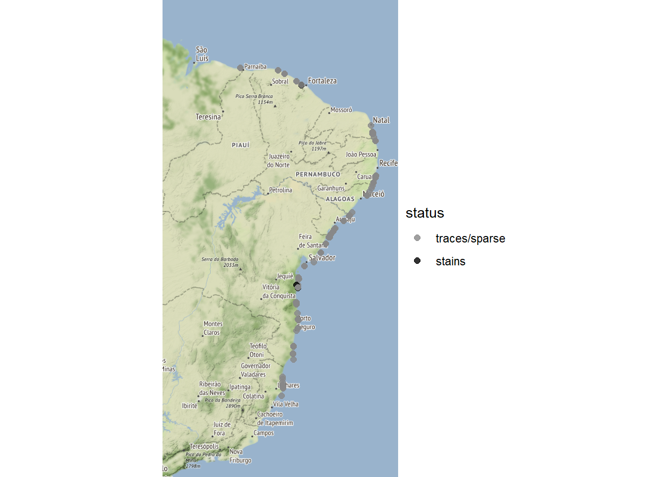
With the data in hand, we’ll try to visualize the communities affected by the oil spill placing the data in a map. There are several frameworks for plotting maps in R, in this post we will use the ggmap package, which we already have used previously in the past.
Before to use ggmap, we’ll need to get the Google Map API Key and register it, but the procedure is pretty straightforward, just following these instructions. In my code, I always store the keys and others sensible information in yalm files to avoid accidentaly publish then in the GitHub, I also commented about this strategy in a older post.
|
|

The animation
Now the last step is to animate the map in the time dimension, we’ll do this using the great gganimate package, adding a transition function in the ggplot2 + ggmap stack.
|
|

Visualizing the spill evolution in one plot
The animated map view gives us an great idea of the size of the ecological impact of the oil spill off the coast of Brazil. But to analytical purpose the animation does not allow you to see the full evolution history at one same time, allowing us to gauge how the spill is progressing.
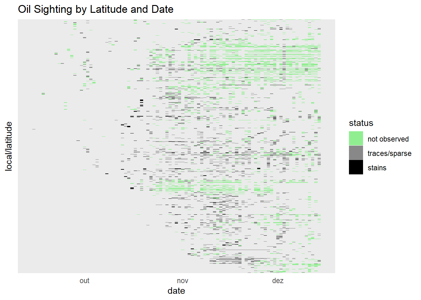
To do this trick, let’s plot the information as a heatmap, where each location will be on the Y axis, indexed by its latitude, and on the X axis we’ll use the date information.
|
|

In this graph, we can visualize how the the oil spill are progressing to the south, following the maritime currents, over the months of October and November, reaching the most extreme point a few days, before December.
The intermittent nature of the chart shows that information registring is not done daily in all locations, and some communities has more status updates than others we should handle this caracteristic to correctly plot the information, but we’ll leave this to other post.