Comparing Fitbit and Polar H7 heart rate data

Giuliano Sposito included in data science

2019-03-05 2888 words 14 minutes

/2019-03-05-comparing-fitbit-and-polar-h7-heart-rate-data/images/fitbit_polar_cover.jpg

Contents

How good is the Fitbit measures comparing to Polar H7? The wearable Fitbit bracelet measures the heart rate based on the expansion and contraction of the capillaries in the skin throught measurement of the reflection and absorption of LED lights, different from the method used heart rate monitor Polar H7, which captures the electrical signals from the heart beat. In this post, we’ll access a WebAPI using OAuth2.0 to get Fitbit data and compare it with those obtained by a Polar H7, imported from a GPX file during the same training session.

Introduction

In this post we will compare acquisition of heart rate data performed by two different devices in the same session training: a sport wearable wristband called Fitbit and a Polar heart monitoring.

How good is the Fitbit measures comparing to Polar H7? They agree with the measures? How the differences are distributed? I did a MTB session using both devices, now I can use R to access the data and compare the measures.

The devices

Fitbit Charge HR

The bracelet model used was Fitbit ChargeHR, which is no longer marketed, but use the same technology embedded in newer models. The Fitbit uses a proprietary technology called PurePulse a to perform a heart rate measurement. When your heart beats, yours capillaries in the skin expand and contract based on changes in blood volume. The light of the PurePulse LEDs on your Fitbit device reflect on the skin to detect changes in blood volume, and finely tuned algorithms are applied to measure heart rate automatically and continuously.

Polar H7

The heart rate monitor used was Polar H7 Heart Rate Sensor, which works as an Electrocardiogram, or in other words, electrodes in contact with the skin detect the electrical signal triggered by the heart in each heart beat.

In this way we will compare the quality and accuracy of heart rate data obtained from two very different technologies.

Data Acquisitions

The first steps is to get the devices data, and for each one we will use a different strategy, for Fitbit we’ll access the data via Web API, and for the Polar H7 we’ll extract from the training session GPX file.

Fitbit

The Fitbit data is availabe throught an Web API in the Fitbit’s Development Portal. It’s necessary to use Oauth 2.0 protocol for authorization and authentication, so you must obtain an ID and Secret doing a registration in the portal first.

Follow the steps:

Log in and go to Manage > Register An App
enter whatever you want for Application name and description
in the application website box, any valid URL (usually I create a link from a google doc)
for organization put “self”
for organization website any valid URL
for OAuth 2.0 Application Type select “Personal”
for Callback URL put in http://localhost:1410/
for Default Access Type select “Read Only”
click “save”

After that, you should now be at a page that shows your

The App Name you choose
OAuth 2.0 Client ID
Client Secret
URL Callback you defined
Authentication URL
Refresh Token URL

These parameters will be used to get or renew the API Access Token. Fill a fitbit_config.yml configuration file (see the appendix at the end of this post) with them and we’ll be ready to request and get the Fitbit data using the httr package.

 1
 2
 3
 4
 5
 6
 7
 8
 9
10


# loading ID and Secret 
# (see the post apendix)
library(yaml)
.config <- yaml.load_file("./config/fitbit_config.yml")

# performing authentication and autorization
library(httr)
fb_app   <- oauth_app(.config$app_name, .config$client_id, .config$client_secret)
fb_oauth <- oauth_endpoint(authorize = .config$auth_uri, access = .config$refresh_token_uri)
token    <- oauth2.0_token(fb_oauth, fb_app, scope = c("activity","heartrate","sleep"), cache = F, use_basic_auth = T)

The oauth_app, oauth_endpoint and oauth2.0_token functions execute the authentication and authorization flow of the OAuth 2.0 protocol to obtain the Access Token, which must be passed for each request made to the Fitbit Web API. When executing these function the browser will be called for you to authenticate in the site, and then the callback URL will be called by passing the authentication token confirming that you have access to the APIs.

Then, we can call the endpoint responsible for querying heart rate information.

 1
 2
 3
 4
 5
 6
 7
 8
 9
10
11
12
13
14
15
16
17
18
19
20
21
22
23
24


# request HR data
# Resource URL - There are two acceptable formats for retrieving time series data:
#
# GET https://api.fitbit.com/1/user/user-id]/activities/heart/date/[date/period.json
# GET https://api.fitbit.com/1/user/user-id]/activities/heart/date/[base-date/end-date.json
#
# user-id:   The encoded ID of the user. Use "-" (dash) for current logged-in user.
# base-date: The range start date, in the format yyyy-MM-dd or today.
# end-date:	 The end date of the range.
# date:	     The end date of the period specified in the format yyyy-MM-dd or today.
# period:	   The range for which data will be returned. Options are 1d, 7d, 30d, 1w, 1m.

# shortcut to define a url to get heart rate
library(glue)
gen_hr_url <- function(.user_id="-",.date="today",.period="1d")
  glue("https://api.fitbit.com/1/user/{.user_id}/activities/heart/date/{.date}/{.period}.json")


# make a HTTP GET 
# 2019-02-24 is the date of my MTB 
resp <- GET(gen_hr_url(.date="2019-02-24"), conf=config(token=token))

# check if the result is 200 (OK)
resp$status_code

1

## [1] 200

If everything went well, the http request returned [status 200](https://www.w3.org/ Protocols / rfc2616 / rfc2616-sec10.html), then we can process the json of the response content to extract the requested heart rate data.

 1
 2
 3
 4
 5
 6
 7
 8
 9
10
11
12
13
14
15
16
17
18
19
20
21
22
23
24
25


# process response content
library(jsonlite)
data <- fromJSON(content(resp, "text"))

# get the heart rate data 
# see the response json format in https://dev.fitbit.com/build/reference/web-api/heart-rate/ 
hrdt <- data$`activities-heart-intraday`$dataset

# convert the "text time data" in in date-time and create a tibble
library(tidyverse)
library(lubridate)
hrdt %>% 
  as.tibble() %>% 
  mutate( datetime = paste0("2019-02-24 ", time) ) %>% # adding "day" to time info
  mutate( datetime = ymd_hms(datetime) ) %>% 
  rename(fitbit_hr = value) %>% 
  select(datetime, fitbit_hr) -> fitbit_hr

# let's see we got
library(knitr)
library(kableExtra)
fitbit_hr %>% 
  head(10) %>% 
  kable() %>%
  kable_styling(bootstrap_options = "striped", full_width = F, font_size = 11)

datetime	fitbit_hr
2019-02-24 00:00:00	73
2019-02-24 00:01:00	70
2019-02-24 00:02:00	70
2019-02-24 00:03:00	72
2019-02-24 00:04:00	77
2019-02-24 00:05:00	74
2019-02-24 00:06:00	77
2019-02-24 00:07:00	72
2019-02-24 00:08:00	73
2019-02-24 00:09:00	70

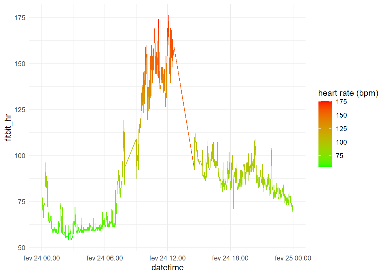
The Fitbit’s heart rate data obtained are minute-by-minute measurements of how much the heart beated, i.e., heart beats per minute, it is possible to plot the heart rate captured by the wearable throughout the day.

1
2
3
4
5
6


# ploting HR x Datatime
fitbit_hr %>% 
  ggplot() +
  geom_line(aes(x=datetime, y=fitbit_hr, color=fitbit_hr)) +
  scale_color_gradient(name="heart rate (bpm)",low="green", high="red") +
  theme_minimal()

Polar H7

Unlike the Fitbit, to access the heart rate data of the Polar H7, the easiest way is to pull the data from the App used in to track the training session, at that time I used the Strava Application connected to the heart monitor by bluetooth. As we did in the post “Ploting your mtb track with R”, we download the GPX file containing the data recorded during the exercise session, directly from the Strava website, and then process the XML to extract the data we are looking for.

 1
 2
 3
 4
 5
 6
 7
 8
 9
10
11
12
13
14
15
16
17
18
19
20
21
22
23
24
25
26
27
28


# read gpx file
library(XML)
gpx_file <- htmlTreeParse("./data/Visconde_de_Sotello_e_Moenda.gpx", useInternalNodes = T)

# trackpoint XML  structure 
#
# <trkpt lat="-22.7036870" lon="-46.7560630">
#   <ele>675.1</ele>
#   <time>2019-02-24T11:13:36Z</time>
#   <extensions>
#     <gpxtpx:TrackPointExtension>
#       <gpxtpx:hr>105</gpxtpx:hr>
#     </gpxtpx:TrackPointExtension>
#   </extensions>
# </trkpt>

# extract (by xpath) times
dtime <- xpathSApply(gpx_file, path = "//trkpt/time", xmlValue) 
hr    <- xpathSApply(gpx_file, path = "//trkpt/extensions/trackpointextension/hr", xmlValue) 

# create a tibble
polar_hr <- tibble(
  datetime  = ymd_hms(dtime),
  polar_hr = as.integer(hr)
)

# overview
summary(polar_hr)

1
2
3
4
5
6
7


##     datetime                      polar_hr    
##  Min.   :2019-02-24 11:13:36   Min.   :101.0  
##  1st Qu.:2019-02-24 12:05:49   1st Qu.:135.0  
##  Median :2019-02-24 13:12:44   Median :143.0  
##  Mean   :2019-02-24 13:12:32   Mean   :144.1  
##  3rd Qu.:2019-02-24 14:24:18   3rd Qu.:154.0  
##  Max.   :2019-02-24 15:17:45   Max.   :180.0

1
2
3
4
5


# lets see the content
polar_hr %>% 
  head(10) %>% 
  kable() %>%
  kable_styling(bootstrap_options = "striped", full_width = F, font_size = 11)

datetime	polar_hr
2019-02-24 11:13:36	105
2019-02-24 11:13:57	105
2019-02-24 11:13:59	101
2019-02-24 11:14:00	102
2019-02-24 11:14:01	103
2019-02-24 11:14:02	103
2019-02-24 11:14:03	103
2019-02-24 11:14:04	103
2019-02-24 11:14:05	104
2019-02-24 11:14:06	103

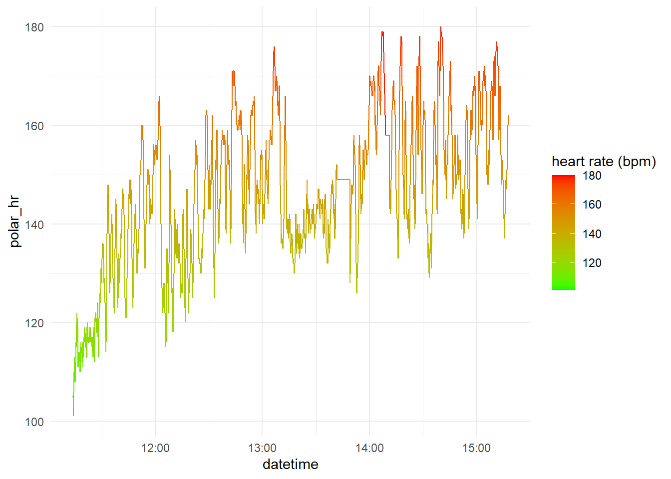
As Fitbit’s data, the heart rate from the Polar H7 obtained are minute-by-minute beats rate, it is possible to visualize the heart rate along the training session.

1
2
3
4
5
6


# Visualize dataset
polar_hr %>% 
  ggplot() +
  geom_line(aes(x=datetime, y=polar_hr, color=polar_hr)) +
  scale_color_gradient(name="heart rate (bpm)",low="green", high="red") + 
  theme_minimal()

Analysis

Comparing measurements

With the dataset at hand, we now can compare the measurements obtained by the two devices. In both measurements, the heart rate is measured in beats per minute and stored minute by minute, let’s join them by timestamp.

 1
 2
 3
 4
 5
 6
 7
 8
 9
10
11
12
13


# join both datasets by the timestamp
# the datetime in polar_hr data are in UTC and the fitbit are in local time
# ajusting the "timezone" and merging both devices removing 2 hours from polar data
polar_hr %>% 
  mutate(datetime = datetime - hours(2)) %>% 
  inner_join(fitbit_hr, by = "datetime") -> hr_data


# let's see what we got
hr_data %>% 
  head(10) %>% 
  kable() %>%
  kable_styling(bootstrap_options = "striped", full_width = F, font_size = 11)

datetime	polar_hr	fitbit_hr
2019-02-24 09:14:00	102	106
2019-02-24 09:15:00	108	109
2019-02-24 09:16:00	117	114
2019-02-24 09:17:00	114	112
2019-02-24 09:18:00	112	113
2019-02-24 09:19:00	113	114
2019-02-24 09:20:00	117	117
2019-02-24 09:21:00	116	116
2019-02-24 09:22:00	118	117
2019-02-24 09:23:00	117	117

Ploting both data toghether.

1
2
3
4
5
6


# lets plot the dataset
hr_data %>% 
  gather(device, hr, -datetime) %>% 
  ggplot(aes(x=datetime, y=hr, group=device)) +
  geom_line(aes(color=device)) +
  theme_minimal()

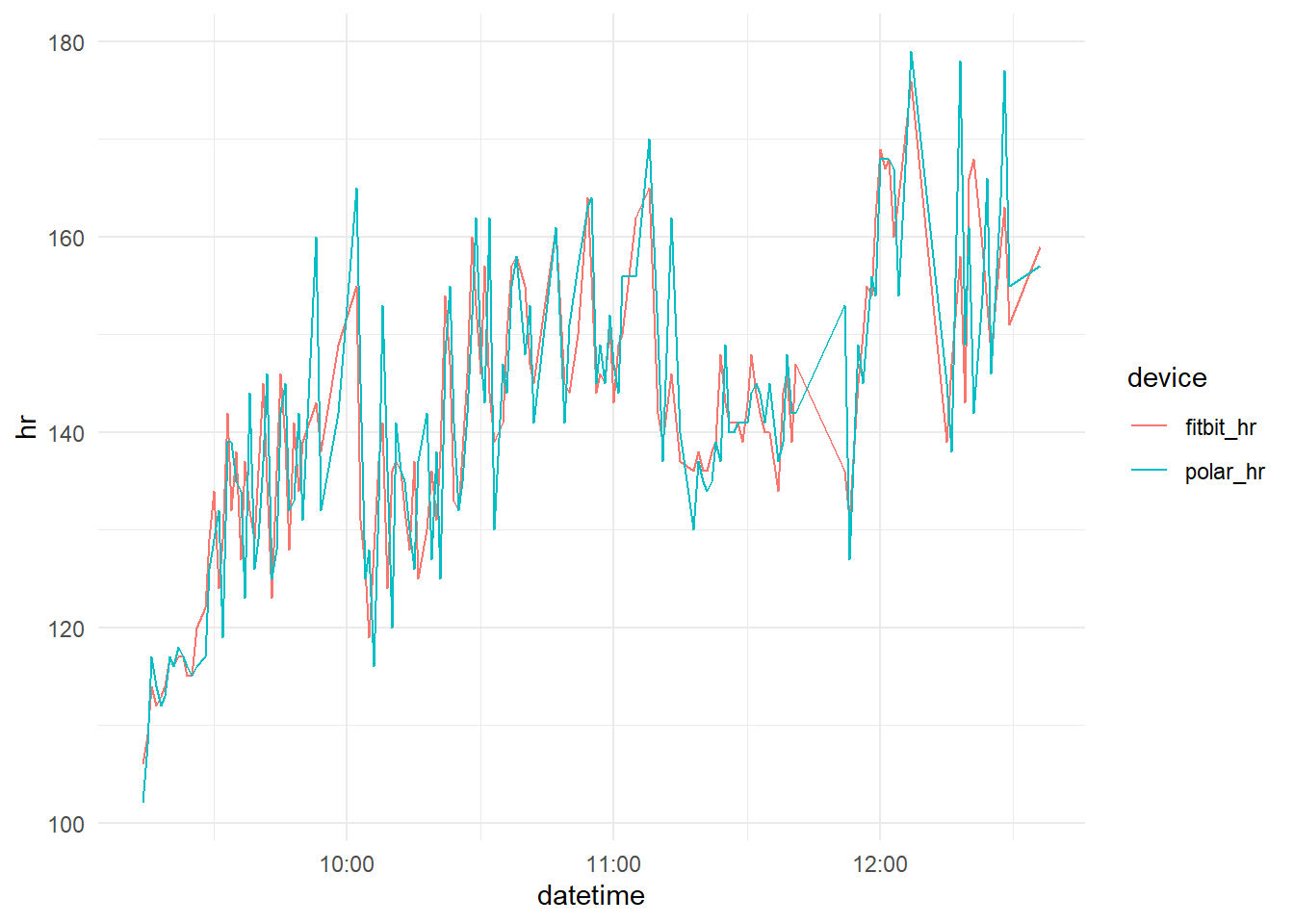
We can see that the measurements of Fitbit follows the Polar H7 data with remarkable proximity, we can better evaluate the relation between them plotting one against other.

1
2
3
4
5
6


# lets see the correlation
hr_data %>% 
  ggplot(aes(x=polar_hr, y=fitbit_hr)) +
  geom_point() +
  stat_smooth(method = "lm") +
  theme_minimal()

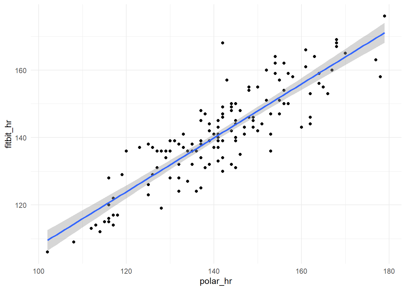
The correlation between the two measurements, although not exactly accurate, is clear, let’s test it

1
2


# correlation test
cor.test(x=hr_data$polar_hr, y=hr_data$fitbit_hr, alternative = "two.sided")

 1
 2
 3
 4
 5
 6
 7
 8
 9
10
11


## 
## 	Pearson's product-moment correlation
## 
## data:  hr_data$polar_hr and hr_data$fitbit_hr
## t = 21.59, df = 143, p-value < 2.2e-16
## alternative hypothesis: true correlation is not equal to 0
## 95 percent confidence interval:
##  0.8301432 0.9082697
## sample estimates:
##       cor 
## 0.8747767

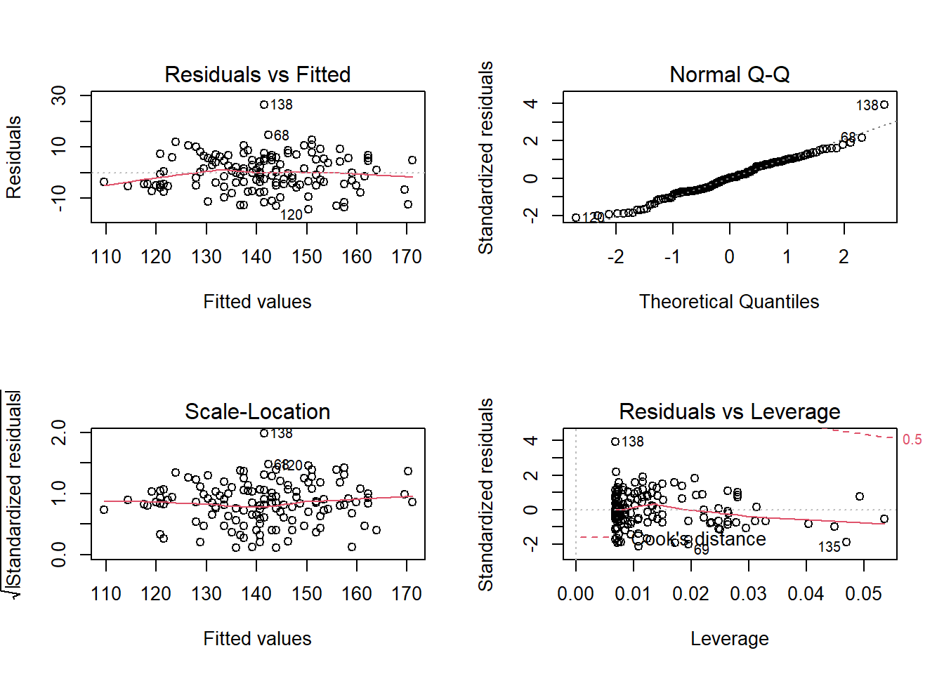
The correlation are 0.87 and significant (p-value < 2.2e-16). We can do the linear regression of the Fitbit measurements on the Polar h7 and analyze how the residues behaves.

1
2
3


# check the quality of a linear correlation
model <- lm(fitbit_hr~polar_hr, hr_data)
summary(model)

 1
 2
 3
 4
 5
 6
 7
 8
 9
10
11
12
13
14
15
16
17
18


## 
## Call:
## lm(formula = fitbit_hr ~ polar_hr, data = hr_data)
## 
## Residuals:
##      Min       1Q   Median       3Q      Max 
## -14.3036  -4.5178   0.0902   4.8933  26.4926 
## 
## Coefficients:
##             Estimate Std. Error t value Pr(>|t|)    
## (Intercept) 27.95671    5.26854   5.306 4.17e-07 ***
## polar_hr     0.79965    0.03704  21.590  < 2e-16 ***
## ---
## Signif. codes:  0 '***' 0.001 '**' 0.01 '*' 0.05 '.' 0.1 ' ' 1
## 
## Residual standard error: 6.763 on 143 degrees of freedom
## Multiple R-squared:  0.7652,	Adjusted R-squared:  0.7636 
## F-statistic: 466.1 on 1 and 143 DF,  p-value: < 2.2e-16

1
2


par(mfrow = c(2, 2))
plot(model)

Bland Altman Agreement Analysis

Bland and Altman published in 1983 the first article as an alternative methodology to the calculation of the coefficient of correlation, methodology used until then. The correlation coefficient does not evaluate agreement and yes association between two measures, very different things.

The methodology initially proposed by Bland and Altman to evaluate the agreement between two variables (X and Y) starts from a graphical view from a dispersion between the difference of the two variables (X - Y) and the average of the two (X + Y) / 2.

Let’s reproduce the methodology with these data.

 1
 2
 3
 4
 5
 6
 7
 8
 9
10
11
12
13
14
15
16
17


# math for Bland Altman test
hr_data %>% 
  mutate(
    mean      = (polar_hr + fitbit_hr)/2,
    diff      = fitbit_hr - polar_hr,
    diff.pct  = (fitbit_hr - polar_hr)/polar_hr,
    diff.mn   = mean(diff),
    diff.sd   = sqrt(var(diff)),
    upper.lim = diff.mn + (2*diff.sd), 
    lower.lim = diff.mn - (2*diff.sd),
  ) -> hr_data_ba

# let's see
hr_data_ba %>% 
  head(10) %>% 
  kable() %>%
  kable_styling(bootstrap_options = "striped", full_width = F, font_size = 11)

datetime	polar_hr	fitbit_hr	mean	diff	diff.pct	diff.mn	diff.sd	upper.lim	lower.lim
2019-02-24 09:14:00	102	106	104.0	4	0.0392157	-0.3793103	7.396573	14.41384	-15.17246
2019-02-24 09:15:00	108	109	108.5	1	0.0092593	-0.3793103	7.396573	14.41384	-15.17246
2019-02-24 09:16:00	117	114	115.5	-3	-0.0256410	-0.3793103	7.396573	14.41384	-15.17246
2019-02-24 09:17:00	114	112	113.0	-2	-0.0175439	-0.3793103	7.396573	14.41384	-15.17246
2019-02-24 09:18:00	112	113	112.5	1	0.0089286	-0.3793103	7.396573	14.41384	-15.17246
2019-02-24 09:19:00	113	114	113.5	1	0.0088496	-0.3793103	7.396573	14.41384	-15.17246
2019-02-24 09:20:00	117	117	117.0	0	0.0000000	-0.3793103	7.396573	14.41384	-15.17246
2019-02-24 09:21:00	116	116	116.0	0	0.0000000	-0.3793103	7.396573	14.41384	-15.17246
2019-02-24 09:22:00	118	117	117.5	-1	-0.0084746	-0.3793103	7.396573	14.41384	-15.17246
2019-02-24 09:23:00	117	117	117.0	0	0.0000000	-0.3793103	7.396573	14.41384	-15.17246

In this graph, it’s possible to visualize the bias (how much the differences deviate from the zero value) and the error distribution (the dispersion of the points of the differences around the mean), in addition to outliers and tendencies.

From the calculation of bias (d) and its standard deviation (sd) it is possible to reach the limits of agreement: d ± 1,96sd, which must be calculated and included in the graph. If the bias presents normal distribution, these limits represent the region where 95% of the differences in the studied cases are found.

1
2
3
4
5
6
7
8
9


# Bland Altman plot
hr_data_ba %>% 
  ggplot(aes(x=mean, y=diff)) + 
  geom_point() +
  geom_hline(yintercept=0, color="grey") +
  geom_hline(yintercept=hr_data_ba$diff.mn[1], linetype=2, color="blue") +
  geom_hline(yintercept=hr_data_ba$upper.lim[1], linetype=2, color="red") +
  geom_hline(yintercept=hr_data_ba$lower.lim[1], linetype=2, color="red") +
  theme_minimal()

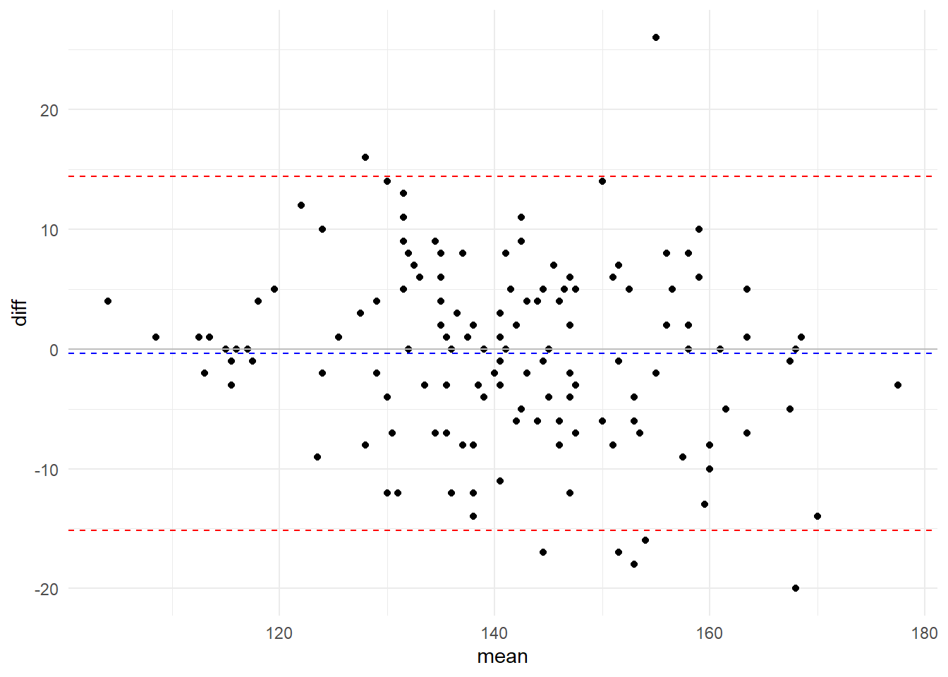
Visually we see that there is no bias (average of the differences is close to zero) and that the dispersion of the differences are within a very small range:

Bias: -0.3793103
Dispersion ($2\sigma$): 14.4138355 bpm

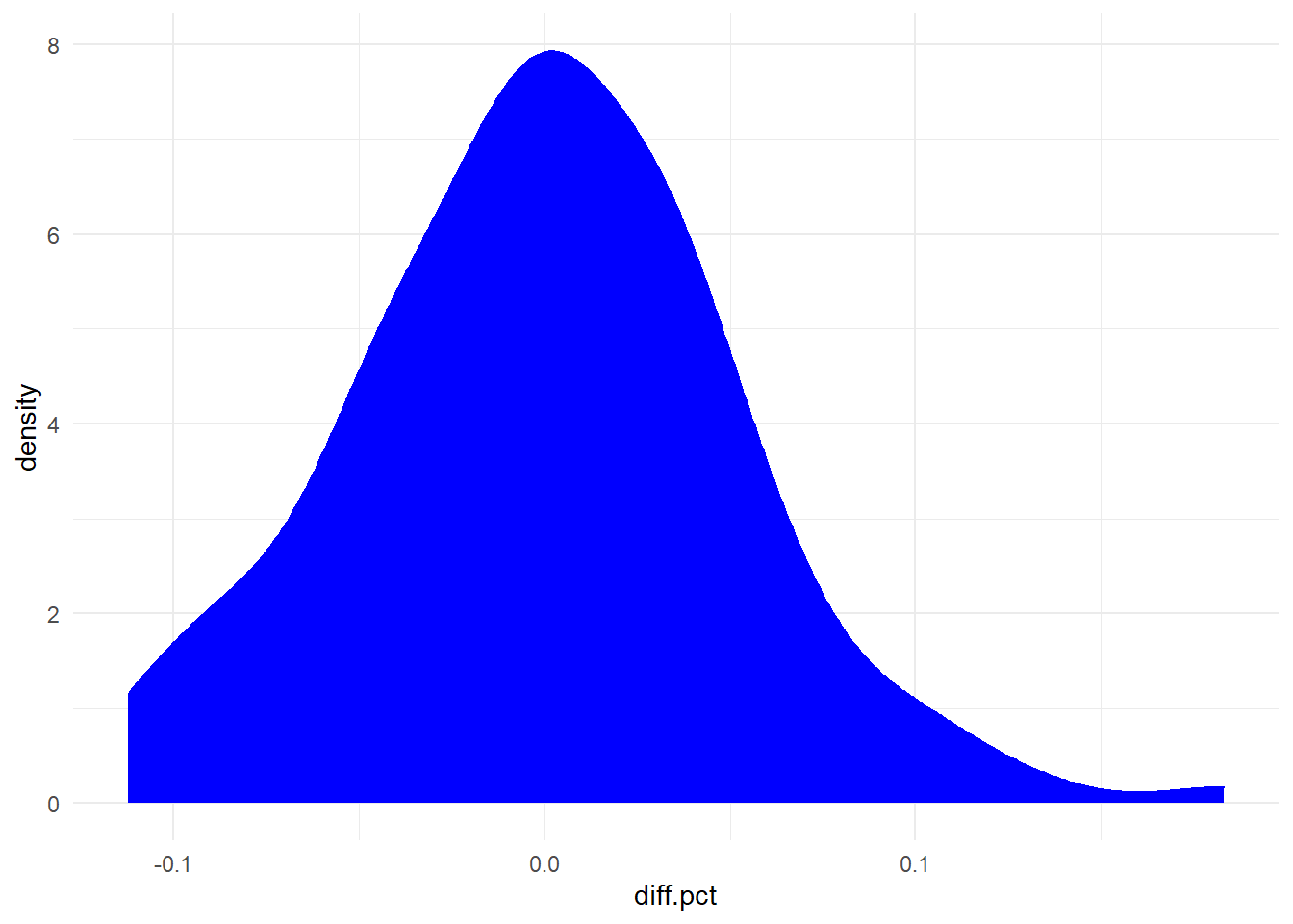
Before proceeding with the analysis, let’s take a look at the distribution of the differences in measurements of fitbit relative to polar h7:

1
2


# Overview
summary(hr_data_ba$diff.pct)

1
2


##       Min.    1st Qu.     Median       Mean    3rd Qu.       Max. 
## -0.1123596 -0.0344828  0.0000000 -0.0004492  0.0324675  0.1830986

1
2
3
4
5


# Visualizing
hr_data_ba %>% 
  ggplot() +
  geom_density(aes(x=diff.pct), color="blue", fill="blue" ) +
  theme_minimal()

For the Bland-Altman test, what should be evaluated is whether the differences between the variables depend on the measurement size or not. This can be done through a correlation between differences and averages, which should be null.

1
2


# correlation between diff and mean
cor.test(x=hr_data_ba$mean, y=hr_data_ba$diff, alternative = "two.sided")

 1
 2
 3
 4
 5
 6
 7
 8
 9
10
11


## 
## 	Pearson's product-moment correlation
## 
## data:  hr_data_ba$mean and hr_data_ba$diff
## t = -2.2191, df = 143, p-value = 0.02806
## alternative hypothesis: true correlation is not equal to 0
## 95 percent confidence interval:
##  -0.3354834 -0.0200386
## sample estimates:
##        cor 
## -0.1824519

Our numbers showed some correlation, where it should not be found, even with the large p-value. The bias hypothesis may or may not be equal to zero can be tested by a t-test for paired samples.

1
2


# t.test between paired samples
t.test(x=hr_data_ba$mean, y=hr_data_ba$diff, paired = T)

 1
 2
 3
 4
 5
 6
 7
 8
 9
10
11


## 
## 	Paired t-test
## 
## data:  hr_data_ba$mean and hr_data_ba$diff
## t = 99.873, df = 144, p-value < 2.2e-16
## alternative hypothesis: true difference in means is not equal to 0
## 95 percent confidence interval:
##  138.8213 144.4270
## sample estimates:
## mean of the differences 
##                141.6241

Here, the bias was practically zero, demonstrating agreement between the measurements of Fitbit and Polar H7.

Conclusion

In this post we use the httr package to access a WebAPI using OAuth2.0 to get data from Fitbit and compare it with that obtained by a Polar H7, imported from a GPX file

The fitbit captures the heart rate based on the expansion and contraction of the capillaries in the skin and makes this measurement based on the reflection / absorption of LED lights. This method proved to be comparable and in agreement with the measurements obtained in the Polar H7 heart monitor, which captures the electrical signals of the beat.

Apendix

config.yml

To prevent passwords, IDs and secrets from being hard coded and getting versioned and exposed in Github accidentally, I usually create a yaml file and put it in .gitignore. In this code, the yaml file has the following format:

 1
 2
 3
 4
 5
 6
 7
 8
 9
10


# registe a new app in Fitbit developer site at # https://dev.fitbit.com/apps/new
# follow the instruction on https://hydroecology.net/getting-detailed-fitbit-data-with-r/
# fill these var contents and save as 'fitbit_config.yml'

app_name: ""
client_id: ""
client_secret: ""
callback_url: ""
auth_uri: ""
refresh_token_uri: ""

References

References used in this post: