Power Analysis | Introduction in R

This post explore Power Analysis technique. Power is the probability of detecting an effect, given that the effect is really there. In other words, it is the probability of rejecting the null hypothesis when it is in fact false. For example, let’s say that we have a simple study with drug A and a placebo group, and that the drug truly is effective; the power is the probability of finding a difference between the two groups.¹

Introduction

So, imagine that we had a power of .8 and that this simple study was conducted many times. Having power of .8 means that 80% of the time, we would get a statistically significant difference between the drug A and placebo groups. This also means that 20% of the times that we run this experiment, we will not obtain a statistically significant effect between the two groups, even though there really is an effect in reality.

Perhaps the most common use is to determine the necessary number of subjects needed to detect an effect of a given size. Note that trying to find the absolute, bare minimum number of subjects needed in the study is often not a good idea. Additionally, power analysis can be used to determine power, given an effect size and the number of subjects available. You might do this when you know, for example, that only 75 subjects are available (or that you only have the budget for 75 subjects), and you want to know if you will have enough power to justify actually doing the study. In most cases, there is really no point to conducting a study that is seriously underpowered.

Besides the issue of the number of necessary subjects, there are other good reasons for doing a power analysis. For example, a power analysis is often required as part of a grant proposal. And finally, doing a power analysis is often just part of doing good research; A power analysis is a good way of making sure that you have thought through every aspect of the study and the statistical analysis before you start collecting data.

Examples

Finding The Sample Size

We’ll apply power analysis in its case more common, to determine the necessary number of subjects to detect a given effect, in this case let’s use the {pwr package} in a scenario of drug treatment. Lets consider a control group and a treatment group to COVID-19, for example. To simplify the case we assume that the recovery time for COVID-19 is normally distributed around 21.91 days (mean) and standard deviation of 5.33 days², how many subjects we will have to had to detect a treatment that can shorter the recovery in 5 days?

 1
 2
 3
 4
 5
 6
 7
 8
 9
10
11
12
13
14
15
16
17
18
19
20
21
22
23
24
25

# install.packages("pwr")
library(pwr)
library(broom)
library(tidyverse)

# covid recovery time (mean and sd)
mo <- 21.91
s0 <- 5.33

# we want to detect 5 day early-recovery time (at same standard deviation) 
mt <- mo-5

# simulation the populations
popCntrl <- rnorm(10000, mo, s0) #control
popTreat <- rnorm(10000, mt, s0) #under treatment

# lets see the populations 
data.frame(
  recoveryTime = c(popCntrl, popTreat),
  group = rep(c("control","popTreat"), each=10000)
) %>%
  ggplot(aes(x=recoveryTime, fill=group, group=group))+
  geom_histogram(alpha=.5, position = 'identity') +
  theme_minimal() +
  labs(title = "Population Distribuition", subtitle = "Comparing control group and treatment group")

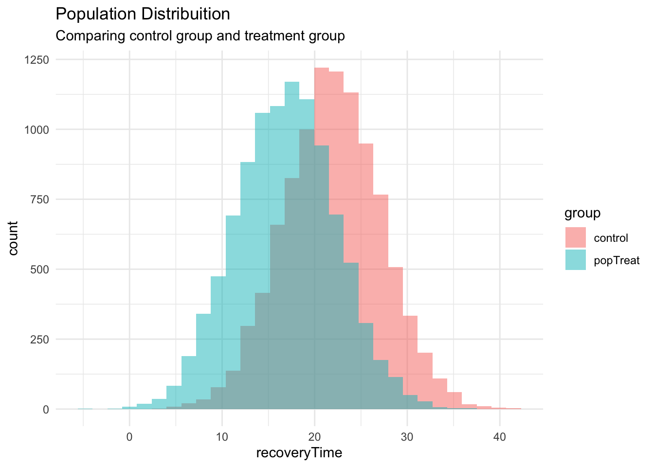
We genarated two different populations which the size of mean difference is well evident, lets do a power analysis to define the sample size necessary to detect this mean difference (~5 days).

To do this, we have to calculate the effect size parameter, in this case we use the mean difference itself measure as standard deviations of the population (a compounded standard deviation of two population, but in this case, to simplify, lets consider the same in both population)³.

So the effect size formula is:

$$ d=\frac{|\mu_{control}-\mu_{popTreat}|}{\sigma} $$

where $ \mu $ are the respective group means and $ \sigma $ is the common standard deviation. So we can use the {pwr} package to calculate the required sample size to reject the null hypothesis with a 80% of statistical power.

1
2
3
4
5
6
7
8

# size efect 21.91 to 16.91
# in this case (simple t.test) the effect size is the mean difference in
# standard deviations (like z-score)
es <- (mo-mt)/s0

# Power Analysis 
pa <- pwr.t.test(sig.level = 0.05, power = .8, d = es)
pa

 1
 2
 3
 4
 5
 6
 7
 8
 9
10

## 
##      Two-sample t test power calculation 
## 
##               n = 18.84853
##               d = 0.9380863
##       sig.level = 0.05
##           power = 0.8
##     alternative = two.sided
## 
## NOTE: n is number in *each* group

We get the minimal sample size to this case as 19 indicated by the parameter n in the return value. Lets check:

1
2
3
4
5
6
7

# samples from control and treatment groups
smpC <- sample(popCntrl, ceiling(pa$n))
smpT <- sample(popTreat, ceiling(pa$n))

# perform a hypothesis test
t <- t.test(smpT, smpC)
t

 1
 2
 3
 4
 5
 6
 7
 8
 9
10
11

## 
## 	Welch Two Sample t-test
## 
## data:  smpT and smpC
## t = -2.193, df = 26.52, p-value = 0.03727
## alternative hypothesis: true difference in means is not equal to 0
## 95 percent confidence interval:
##  -8.2565512 -0.2710736
## sample estimates:
## mean of x mean of y 
##  16.77456  21.03837

As you see, we can test the hypothesis with a p.value of 0.0373, showing that the two sample came indeed from different populations.

To understand this analysis, lets see how the p.value behavior in this case, for different samples sizes (something like to a p.hacking):

 1
 2
 3
 4
 5
 6
 7
 8
 9
10
11
12
13
14
15
16
17
18
19
20
21
22
23
24
25
26
27
28
29

# different samples to check how p.value behaviors 
# from 3 (minimal) to the power analysis sujestions (and more 2)
n_samples <- 3:(ceiling(pa$n)+2)

# for each sample size we perform a hypothesis test 100 times
# we are interesting in the 'p.value' distribution 
iter.tests <- 1:100 %>% 
  map_df(function(.i){
    # for each sample size 
    n_samples %>% 
      map_df(function(n){
      t.test(sample(popCntrl,n), sample(popTreat,n)) %>% 
        tidy() %>% 
        select(p.value) %>% 
        mutate(sample_size=n) %>% 
        return()
      }) 
  })

# ploting the p.values distribution along each sample size
iter.tests %>% 
  ggplot(aes(x=as.factor(sample_size), y=p.value)) +
  geom_boxplot() +
  geom_hline(yintercept = 0.05, color="red", linetype="dashed")+
  theme_minimal() + 
  labs(title = "Sample size effect in P-Value",
       subtitle = "P-Value distribution in 100 t.test at different samples sizes",
       y = "p.value distribution",
       x = "sample size")

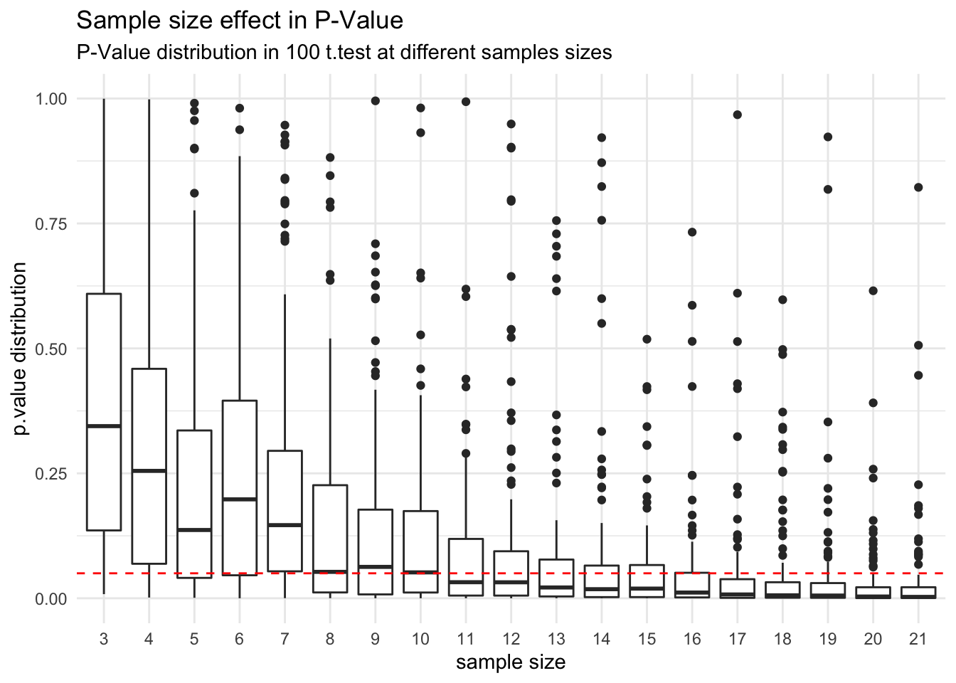
You can see that the hypothesis test of two samples comming from different populations, start to indicate a statistical significance of 0.05 to reject the null hypothesis when the sample size get close the number suggested by the power analysis (19), also we can check the frequency which a t.test finds statistical significance for each sample size.

 1
 2
 3
 4
 5
 6
 7
 8
 9
10
11
12
13
14
15
16
17
18
19

# lets count (for each sample size) in how many of the 100 trials
# we obtain a statistical significance (pvalue <= 0.05)
iter.tests %>% 
  mutate( rejected = p.value <=0.05 ) %>% 
  count(rejected, sample_size) %>% 
  mutate(n=n/100) %>% # pct
  filter(rejected==T) %>% 
  # lets see the proportion 
  ggplot(aes(x=sample_size, y=n)) +
  # power parameter 
  geom_hline(yintercept = pa$power, color="red", linetype="dashed" ) +
  # sample size to detect the desired effect size at 80% of power
  geom_vline(xintercept = ceiling(pa$n), color="red", linetype="dashed") +
  geom_point() + 
  ylim(0,1) +
  theme_minimal() +
  labs(title = "Power",
       subtitle="Probability that your test will find a true statistically significant",
       x="sample size", y="power")

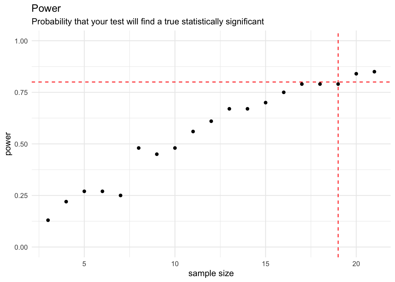
The frequency that a t.test can get 0.05 as p.value to reject the null hypothesis surpass 80% (power parameter) when the sample size pass 19, as expected, once we perform the power analysis with 0.8 as power parameter.

What effect size we can detect in a situation?

Another way to use the power analysis is to find, at some conditions or research scenario, which is the smaller effect size we can detect with (with statistical significance). For example, in the same scenario above, for a COVID-19 recovery time ($ \mu=21.9, \sigma=5.33 $ ), if researchers run a trial for a drug with 50 subjects, 25 in control and 25 in treatment, what is the smaller effect size we could detect?

Using the same package and function, but now, passing in the parameters the sample size and not de effect size:

1
2
3

# Power Analysis 
pa2 <- pwr.t.test(sig.level = 0.05, power = .8, n=25)
pa2

 1
 2
 3
 4
 5
 6
 7
 8
 9
10

## 
##      Two-sample t test power calculation 
## 
##               n = 25
##               d = 0.8087121
##       sig.level = 0.05
##           power = 0.8
##     alternative = two.sided
## 
## NOTE: n is number in *each* group

So, we get the effect size that we can statistically detect of a value 0.938, that in this case represents 5 days of recovery ($ h*\sigma $).

Conclusion

Power Analysis perform an important role in a statistical research, we can use this technique to avoid p.hacking defining the research parameters before it happens, to enforce our conclusions and filter bias.

To be continued

In the next post, we’ll explorer a use case for power analysis taken from Matthew J. Salganik’s book Bit by Bit: Social Research in the Digital Age shows how difficult it is to measure the return on investment of online ads, even with digital experiments involving millions of customers.

References