We learn from the masters, doing the math by ourselves, so, in this post we reproduce two data analysis from David Robinson’s #TidyTuesday screencasts, the first one about the horro movie ratings dataset where he uses a lasso regression to predict the ratings of a movie based on genre, cast and plot. The second is about a dataset of pizza ratings in NYC and other cities. There are goods data handling tricks using tidyverse in these analysis.
In this post we reproduce two data analysis from David Robinson’s#TidyTuesday screencasts, the first one about the horror movie ratings dataset where he uses a lasso regression to predict the ratings of a movie based on genre, cast and plot. The second is about a dataset of pizza ratings in NYC and other cities.
In this #tidytuesday screencast, I analyze a dataset of horror movie ratings, and use lasso regression to predict ratings based on genre, cast, and plot.
# basic setuplibrary(tidyverse)library(knitr)# for kablelibrary(kableExtra)# to change tables font sizelibrary(glue)theme_set(theme_minimal())# changing ggplot2 default theme# data loadhorror_movies_raw<-readr::read_csv("https://raw.githubusercontent.com/rfordatascience/tidytuesday/master/data/2019/2019-10-22/horror_movies.csv")glimpse(horror_movies_raw)
We see here, besides a release_date attribute, there is also a year information inside the title field, let’s extract this data into a new year column. Also, we have to correctly parsing the budget column. Note that the plot column also has a strange content.
1
horror_movies_raw[1,]$plot
1
## [1] "Directed by Elias. With Jason Vail, Nicholas Wilder, Sarah Schoofs, Kirstianna Mueller. Family man Tom has seen something he can't forget, a mysterious video with an ugly secret that soon spreads into his daily life and threatens to dismantle everything around him."
It starts with the director of the movie, the cast and only after that the movie plot, we need to split these infos in diferent columns.
 1
 2
 3
 4
 5
 6
 7
 8
 9
10
11
# some data cleaninghorror_movies<-horror_movies_raw%>%arrange(desc(review_rating))%>%# remove the "year" from title and put into a "year" columnextract(title,"year","\\((\\d\\d\\d\\d)\\)$",remove=F,convert=T)%>%# using "parse_number" to correctly the buget columnmutate(budget=parse_number(budget))%>%# Splitting the "plot" info. We split each sentence in diferent columns.# First one to the director, one for the actors and the remaings to the "plot"separate(plot,c("director","cast_sentence","plot"),sep="\\. ",extra="merge",fill="right")%>%distinct(title,.keep_all=T)
# how much movies by genres?horror_movies%>%count(genres,sort=T)%>%head(10)%>%kable()
genres
n
Horror
1048
Horror| Thriller
469
Comedy| Horror
245
Horror| Mystery| Thriller
171
Drama| Horror| Thriller
159
Drama| Horror
72
Horror| Sci-Fi| Thriller
66
Drama| Horror| Mystery| Thriller
53
Action| Horror| Thriller
48
Horror| Mystery
47
1
2
3
4
5
# by languagehorror_movies%>%count(language,sort=T)%>%head(10)%>%kable()
language
n
English
2407
Spanish
94
Japanese
75
NA
70
Hindi
37
Filipino|Tagalog
34
Thai
34
English|Spanish
30
Turkish
29
German
28
1
2
3
4
5
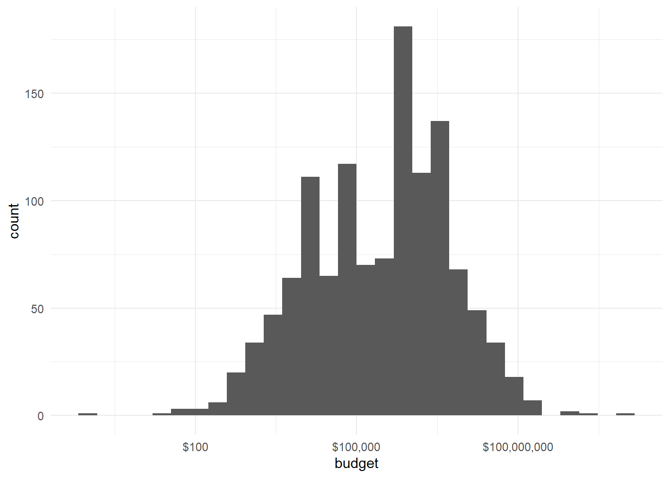
# how is the bugdet distributionhorror_movies%>%ggplot(aes(budget))+geom_histogram()+scale_x_log10(labels=scales::dollar)
One of the things I didn’t know was how to format the datatype in the chart axis, in the screencast David uses the function scales::dollar() to transform the X axis in money. The package Scales map data to aesthetics, and provide methods for automatically determining breaks and labels for axs and legends, pretty handy.
Do higher budget movies end up higher rated?
1
2
3
4
5
6
# plot budget x ratinghorror_movies%>%ggplot(aes(budget,review_rating))+geom_point()+scale_x_log10(labels=scales::dollar)+geom_smooth(method="lm")
No relationshiop between budget and rating. How about movie rating (classification of film’s suitability for certain audiences based on its content) and the movie review (people’s movie evaluation)?
1
2
3
4
5
6
7
8
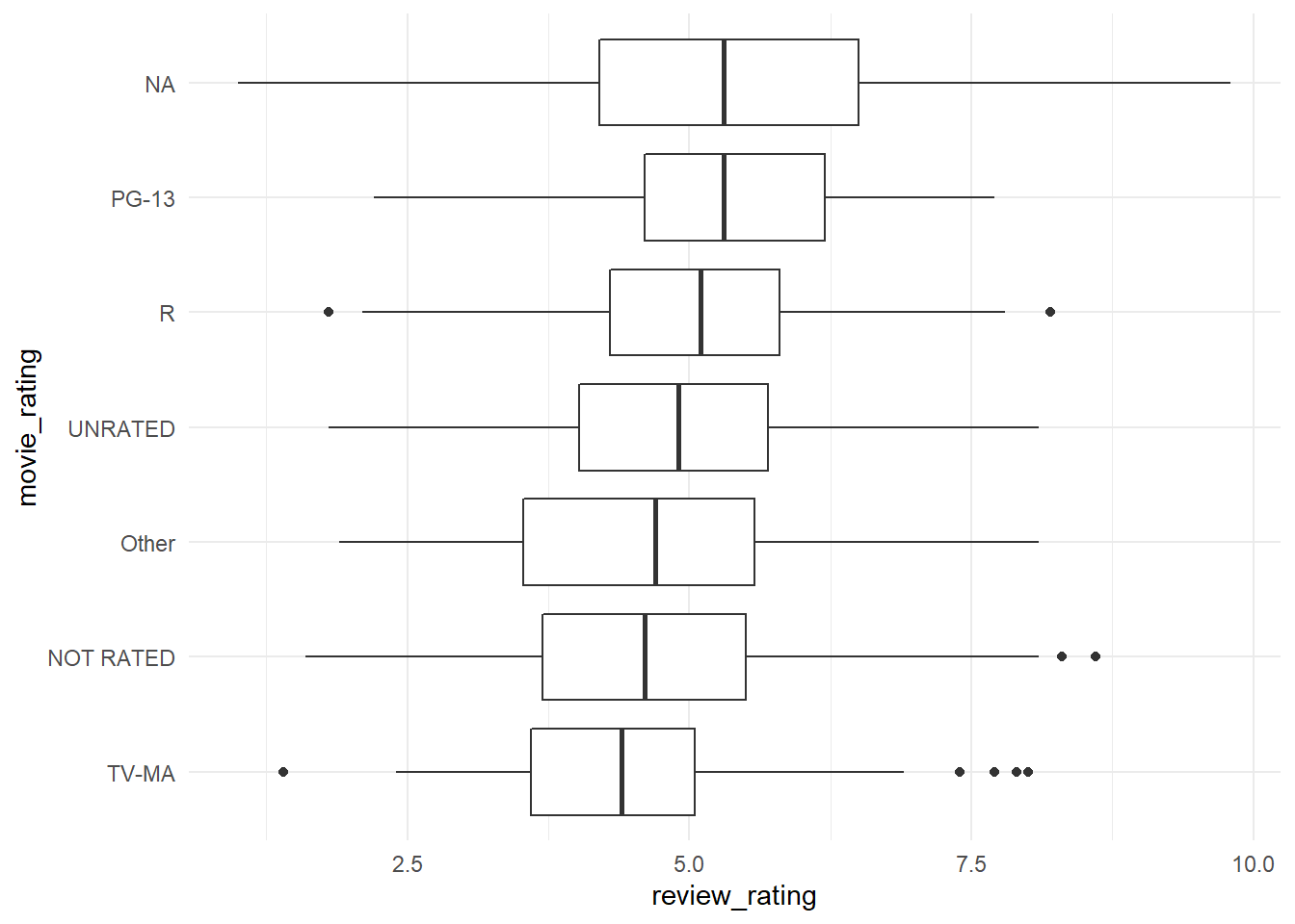
# let's look movie_rating x review_ratinghorror_movies%>%mutate(movie_rating=fct_lump(movie_rating,5),movie_rating=fct_reorder(movie_rating,review_rating,na.rm=T))%>%ggplot(aes(movie_rating,review_rating))+geom_boxplot()+coord_flip()
Two forcats functions were util here, the fct_lump() used to collapse the least frequent values of a factor into “other” and fct_reorder() to reorder the factor movie_rating by another variable, in this case, the median (default function) of movie_rating itself. Doing this we can put the movie_rating in order on the chart.
Seems that there is a relationship between movie_review and movie_rating, how much?
1
2
3
4
5
6
# Calculates the "anova" of Linear Regration between Rating and Reviewhorror_movies%>%filter(!is.na(movie_rating))%>%mutate(movie_rating=fct_lump(movie_rating,5))%>%lm(review_rating~movie_rating,data=.)%>%anova()
1
2
3
4
5
6
7
8
## Analysis of Variance Table
##
## Response: review_rating
## Df Sum Sq Mean Sq F value Pr(>F)
## movie_rating 5 70.05 14.0092 9.1759 1.319e-08 ***
## Residuals 1424 2174.08 1.5267
## ---
## Signif. codes: 0 '***' 0.001 '**' 0.01 '*' 0.05 '.' 0.1 ' ' 1
Let’s plot this in a better way.
 1
 2
 3
 4
 5
 6
 7
 8
 9
10
11
12
13
14
15
16
17
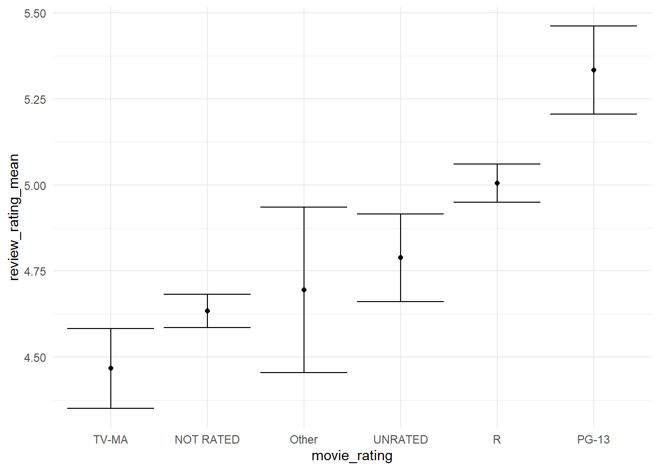
# plotting the mean and standard deviation of movie reviews# for each movie ratinghorror_movies%>%filter(!is.na(movie_rating))%>%mutate(movie_rating=fct_lump(movie_rating,5),movie_rating=fct_reorder(movie_rating,review_rating,na.rm=T))%>%group_by(movie_rating)%>%summarise(review_rating_mean=mean(review_rating,na.rm=T),review_rating_var=var(review_rating,na.rm=T),review_rating_sd=sd(review_rating,na.rm=T),review_rating_error=sqrt(review_rating_var/length(review_rating)))%>%ungroup()%>%ggplot(aes(movie_rating,review_rating_mean))+geom_point()+geom_errorbar(aes(ymin=review_rating_mean-review_rating_error,ymax=review_rating_mean+review_rating_error))
There some preferences, but not too much difference.
Textual Analysis
Let’s explore the plot field throught text analysis. Is there any word that influences the review_rating?
 1
 2
 3
 4
 5
 6
 7
 8
 9
10
11
12
13
14
15
library(tidytext)# to tokenize the plot text# tokenizehorror_movies_unnested<-horror_movies%>%# split tokensunnest_tokens(word,plot)%>%# remove meaningless wordsanti_join(stop_words,by="word")%>%filter(!is.na(word))# lets checkhorror_movies_unnested%>%count(word,sort=T)%>%head(10)%>%kable()
word
n
house
318
friends
313
life
289
family
271
night
256
home
254
woman
244
horror
241
mysterious
234
town
217
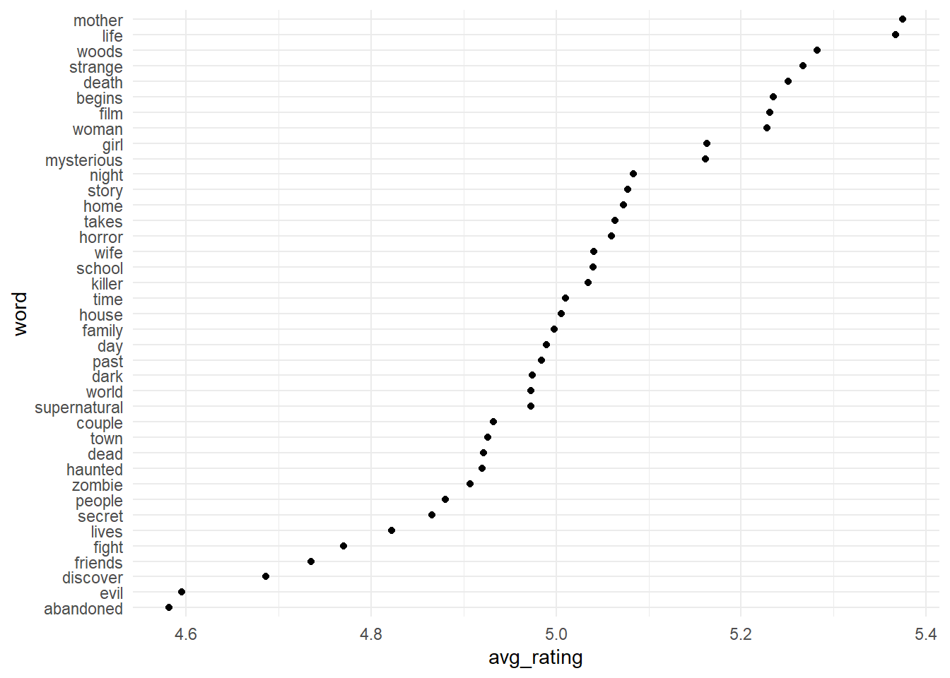
Visualizing word and the average of review_rating.
1
2
3
4
5
6
7
8
9
10
11
12
13
14
15
# Visualizing word and the average of review_ratinghorror_movies_unnested%>%filter(!is.na(review_rating))%>%group_by(word)%>%# by word, count and mean the review_ratingsummarise(movies=n(),avg_rating=mean(review_rating))%>%arrange(desc(movies))%>%# words that appears in the plot of 100 or more movies onlyfilter(movies>=100)%>%mutate(word=fct_reorder(word,avg_rating))%>%ggplot(aes(avg_rating,word))+geom_point()
Lasso Regression for Predicting Review Rating on Words
Lasso stands for Least Absolute Shrinkage Selector Operator, it is a type of regression that allow you to regularize (“shrink”) coefficients. This means that the estimated coefficients are pushed towards 0, to make them work better on new data-sets (“optimized for prediction”). This allows you to use complex models and avoid over-fitting at the same time.
library(glmnet)# lassolibrary(Matrix)# to handle sparse matrixes# word sparse matrixmovie_word_matrix<-horror_movies_unnested%>%filter(!is.na(review_rating))%>%add_count(word)%>%# palavras que apareceram pelo menos 20 vezesfilter(n>=20)%>%count(title,word)%>%# sparse matrixcast_sparse(title,word,n)# let's see how many words aredim(movie_word_matrix)
1
## [1] 2945 460
1
2
3
4
5
# indexing review_rating by the word in the sparse matrixrating<-horror_movies$review_rating[match(rownames(movie_word_matrix),horror_movies$title)]# fitting the LASSO modellasso_model<-cv.glmnet(movie_word_matrix,rating)
Let’s see the characteristics of the fitted model.
1
2
3
4
5
6
7
8
9
10
11
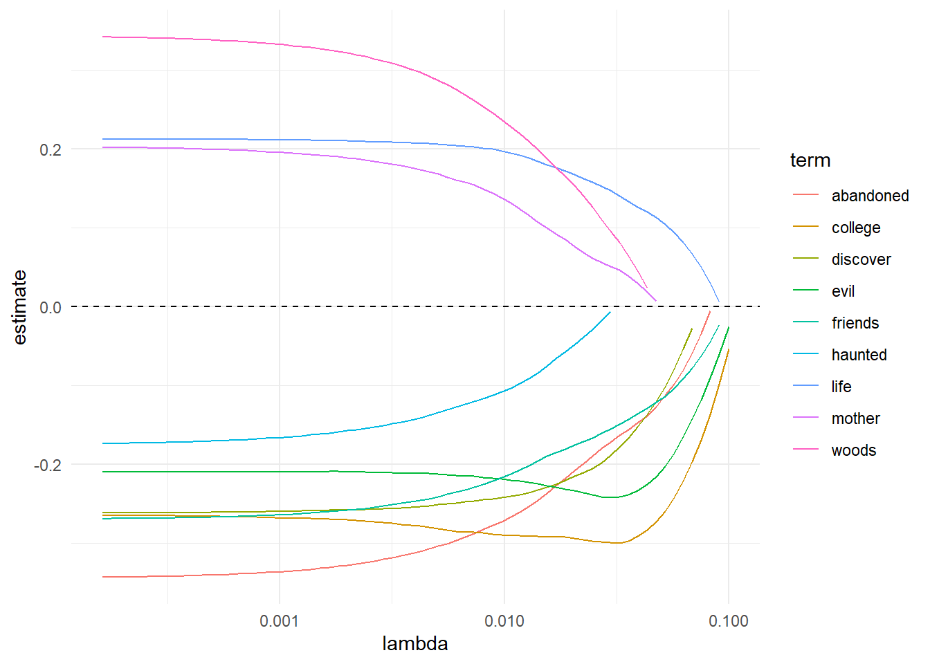
library(broom)# lets see how the coeficient shrink for some "popular" terms# conform the "lambda" term risestidy(lasso_model$glmnet.fit)%>%filter(term%in%c("friends","evil","college","haunted","mother","life","woods","discover","abandoned","woods"))%>%ggplot(aes(lambda,estimate,color=term))+geom_line()+scale_x_log10()+geom_hline(yintercept=0,lty=2)
1
2
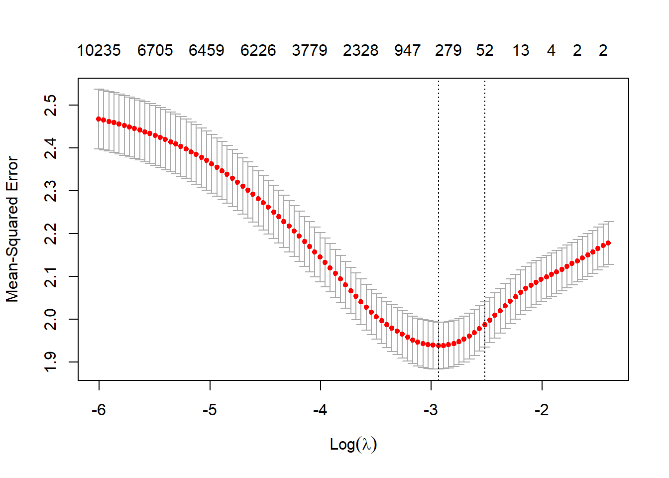
3
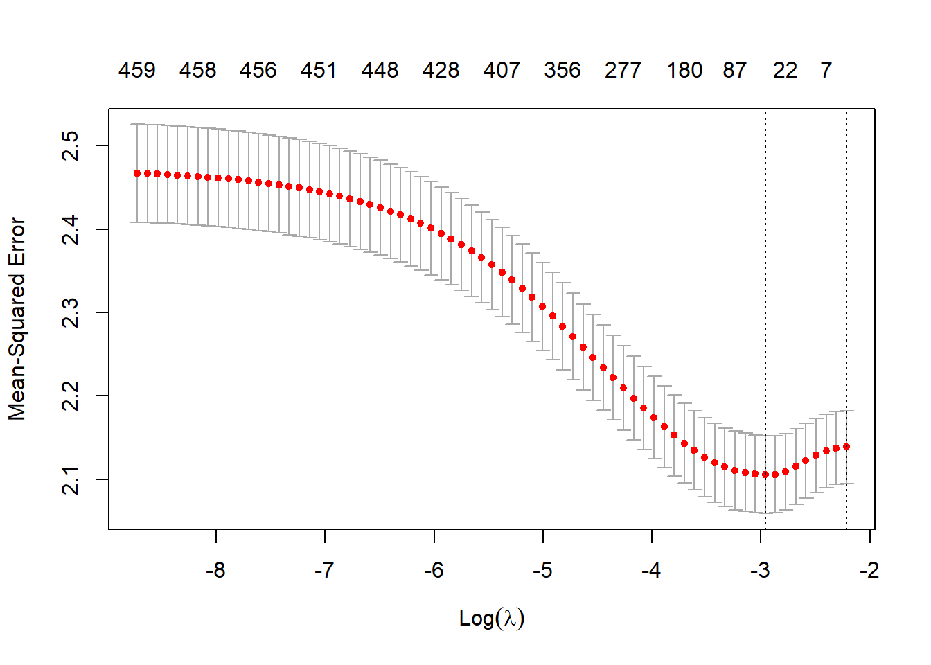
# we are able to visualize the CV performance # in function of lambda parameterplot(lasso_model)
1
2
3
# the model give us the lambda for optimal performance# (min square feet error)log(lasso_model$lambda.min)
1
## [1] -2.958961
1
2
3
4
5
6
7
8
9
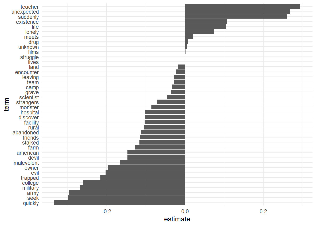
# at that lambda level, let's see how each term# weighted in the modeltidy(lasso_model$glmnet.fit)%>%filter(lambda==lasso_model$lambda.min,term!="(Intercept)")%>%mutate(term=fct_reorder(term,estimate))%>%ggplot(aes(term,estimate))+geom_col()+coord_flip()
1
2
3
4
5
6
7
8
9
10
11
12
13
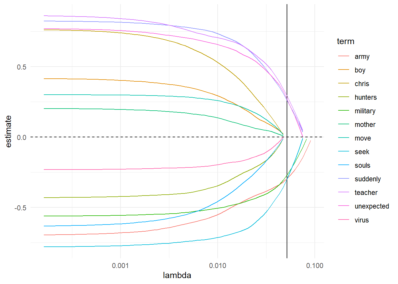
# Let's see how the extrem terms shrink# acording lambdatidy(lasso_model$glmnet.fit)%>%filter(term%in%c("seek","quick","military","army","teacher","unexpected","suddenly",# extremes"boy","move","mother","chris","virus","souls","hunters"# intermediary))%>%ggplot(aes(lambda,estimate,color=term))+geom_vline(xintercept=lasso_model$lambda.min)+geom_line()+scale_x_log10()+geom_hline(yintercept=0,lty=2)
Lasso for words and other features
Throwing everything into a linear model: director, cast, genre, rating, plot and words. David did a “generic” feature generator where he puts in the word sparse matrix other features as “words”, see the code.
# this is a generic feature generatorfeatures<-horror_movies%>%filter(!is.na(review_rating))%>%# features to be addedselect(title,genres,director,cast,movie_rating,language,release_country)%>%# clean director columnmutate(director=str_remove(director,"Directed by "))%>%# transform the info into a key value pair for each movie title# the type is the feature "column"pivot_longer(-title,names_to="type",values_to="value")%>%filter(!is.na(value))%>%# if value field has more than one value (like genres) slip in multiple linesseparate_rows(value,sep="\\| ?")%>%# colapse two columns (type and values) in to column featureunite(feature,type,value,sep=": ")%>%mutate(n=1)movie_feature_matrix<-horror_movies_unnested%>%filter(!is.na(review_rating))%>%count(title,feature=paste0("word: ",word),sort=T)%>%bind_rows(features)%>%cast_sparse(title,feature)dim(movie_feature_matrix)
1
## [1] 3051 46969
With the steps to transform the feature columns in a “key-value pair an then colapse them into a “feature-word”, allow you add and remove features simply changing the select statement in the code above. David uses the convenient tidyr::unite() function to do the concatenation between two columns.
1
2
3
4
5
6
# indexing movie_rating by feature name matrixrating<-horror_movies$review_rating[match(rownames(movie_feature_matrix),horror_movies$title)]# new modelfeature_lasso_model<-cv.glmnet(movie_feature_matrix,rating)plot(feature_lasso_model)
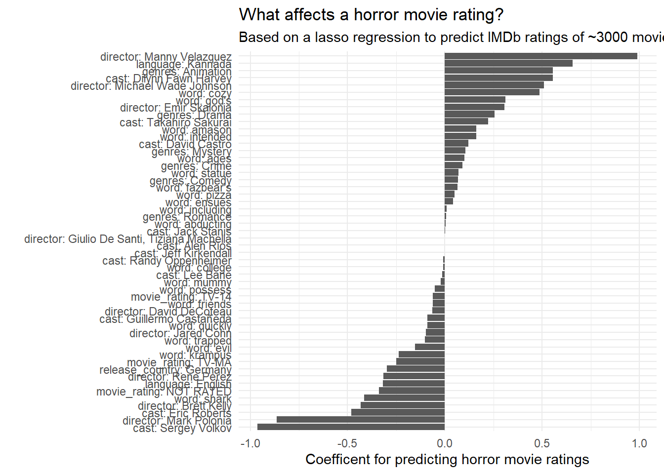
Let’s see what are the most influent features in the lasso regression, but at this time, we’ll see the coenficients at another level than minimal cross validation erro.
In the lasso model object, lambda.min is the value of lambda that gives minimum mean cross-validated error. The other parameter saved is lambda.1se, which gives the most regularized model such that error is within one standard error of the minimum.
To use that, we only need to replace lambda.min with lambda.1se.
1
2
3
4
5
6
7
8
9
10
11
12
# extracting the model coeficientstidy(feature_lasso_model$glmnet.fit)%>%# at lambda.1se levelfilter(lambda==feature_lasso_model$lambda.1se,term!="(Intercept)")%>%mutate(term=fct_reorder(term,estimate))%>%ggplot(aes(term,estimate))+geom_col()+coord_flip()+labs(x="",y="Coefficent for predicting horror movie ratings",title="What affects a horror movie rating?",subtitle="Based on a lasso regression to predict IMDb ratings of ~3000 movies")
What am I going to watch?
The end this analysis, let’s do a simple query to see what horror movie we could watch.
1
2
3
4
5
6
7
8
9
10
11
12
13
14
# lets take the datasethorror_movies%>%filter(# selecting a horror movie that is also a commedystr_detect(genres,"Comedy"),!is.na(movie_rating),!is.na(budget),movie_rating!="PG")%>%arrange(desc(review_rating))%>%select(title,review_rating,plot,director,budget,language)%>%head(5)%>%kable()%>%kable_styling(font_size=10)
title
review_rating
plot
director
budget
language
What We Do in the Shadows (2014)
7.6
A documentary team films the lives of a group of vampires for a few months. The vampires share a house in Wellington, New Zealand. Turns out vampires have their own domestic problems too.
Directed by Jemaine Clement, Taika Waititi
1600000
English|German|Spanish
Only Lovers Left Alive (2013)
7.3
A depressed musician reunites with his lover. Though their romance, which has already endured several centuries, is disrupted by the arrival of her uncontrollable younger sister.
Directed by Jim Jarmusch
7000000
English|French|Arabic|Turkish
Holla II (2013)
6.9
With Vanessa Bell Calloway, Kiely Williams, Greg Cipes, Trae Ireland. After narrowly escaping with her life at the hands of her mentally ill sister Veronica, Monica, with the help of her Mother, Marion, has taken great measures to ensure her safety, including changing her face and relocating to the South. Six years has past and now she finally believes she is safe from Veronica. Little does she know that death and betrayal still await her and her friends on the eve...
Directed by H.M
1000000
English
Wild Men (2017)
6.9
The inept cast and crew of a surprise hit reality-TV show travel deep into the Adirondack mountains for their second season to find proof that Bigfoot exists. Any remaining skepticism they have is ripped to pieces.
Directed by Bobby Sansivero
97948
English
Night Terrors (2014)
6.9
A devious older sister fills her brother's head with bizarre tales of terror, blood soaked memories, and nightmares of perversion after finding out that she has to babysit and miss the party.
Directed by Alex Lukens, Jason Zink
5000
English
Pizza Ratings
In the last #TidyTuesday analysis in this post, we’ll analyze a dataset of pizza ratings, just for fun and because everybody likes pizza. :)
The pizza evaluation datasets are available in the GitHub’s TidyTueday Repo there are three different data sources, let’s see explore one of them.
1
2
3
4
5
6
7
8
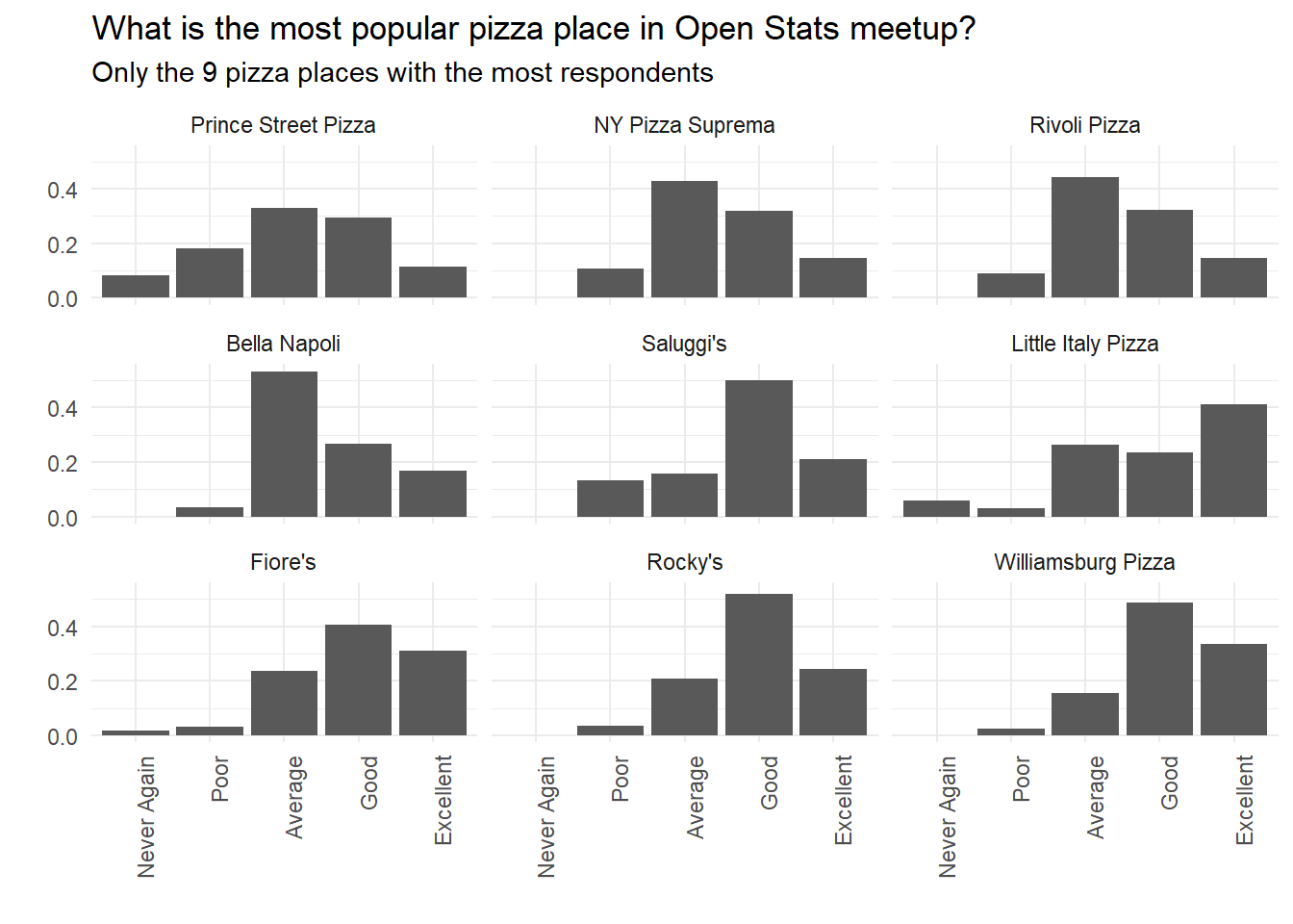
# getting data from githubpizza_jared<-readr::read_csv("https://raw.githubusercontent.com/rfordatascience/tidytuesday/master/data/2019/2019-10-01/pizza_jared.csv")# overal lookpizza_jared%>%head(10)%>%kable()%>%kable_styling(font_size=11)
# by placeby_place_answer%>%# with at least 29 evaluations (cabalistic number to show 9 facets!)filter(total>=29)%>%# controls the order of the facets (worst->better)mutate(place=fct_reorder(place,average))%>%ggplot(aes(answer,percent))+geom_col()+facet_wrap(~place)+theme(axis.text.x=element_text(angle=90,hjust=1))+labs(x="",y="",title="What is the most popular pizza place in Open Stats meetup?",subtitle="Only the 9 pizza places with the most respondents")
David apply a trick to control the number of places that will be show in the plot.
1
2
3
4
5
6
7
8
9
10
11
12
13
14
15
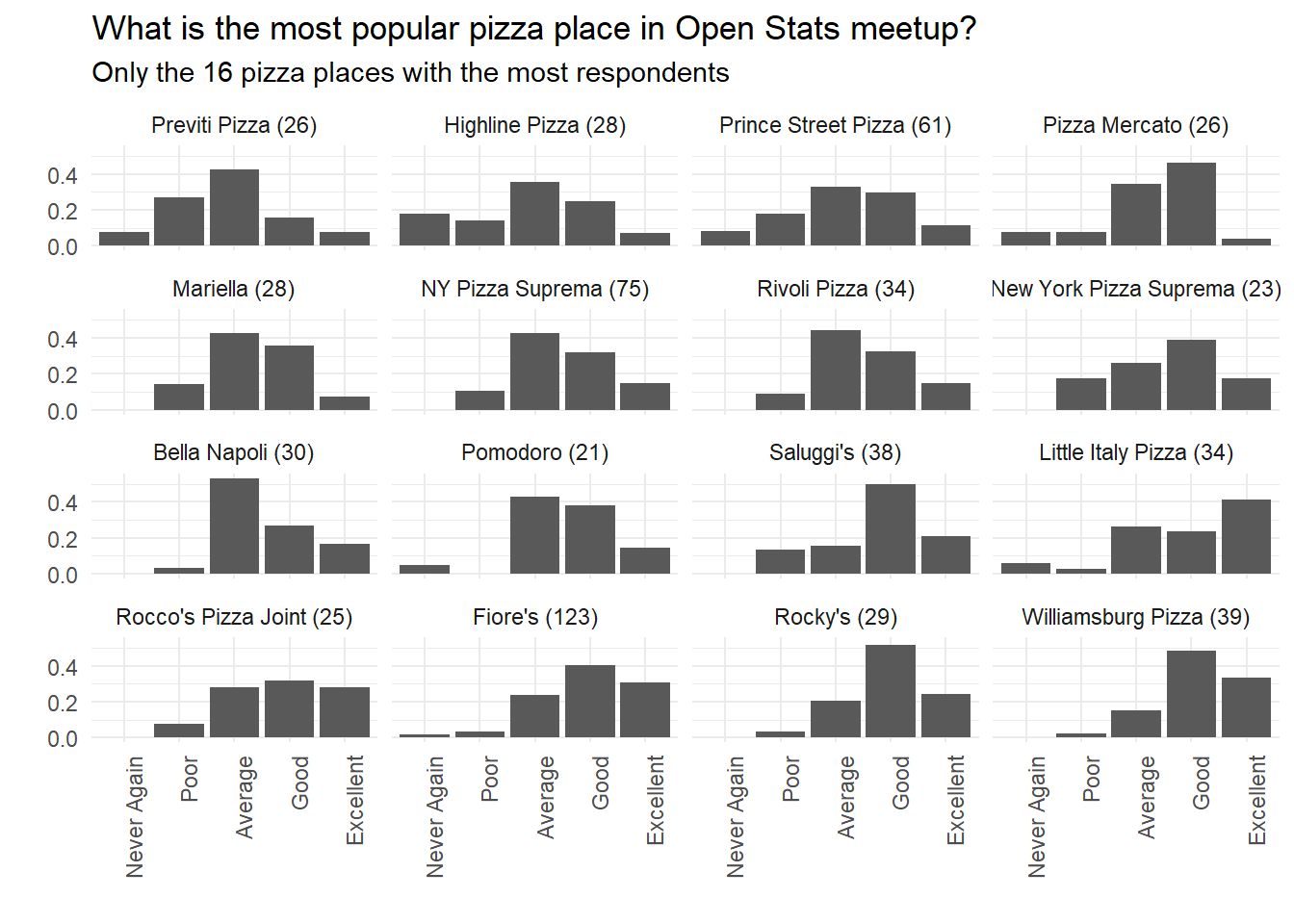
by_place_answer%>%# trick to choose "top N"# reorder by total de votes in reverse order# convert to integer and get "rank" <= Nfilter(as.integer(fct_reorder(place,total,.desc=T))<=16,answer!="Fair")%>%# there just one vote with answer 'fair'mutate(place=glue("{place} ({total})"),# number of samplesplace=fct_reorder(place,average))%>%ggplot(aes(answer,percent))+geom_col()+facet_wrap(~place)+theme(axis.text.x=element_text(angle=90,hjust=1))+labs(x="",y="",title="What is the most popular pizza place in Open Stats meetup?",subtitle="Only the 16 pizza places with the most respondents")
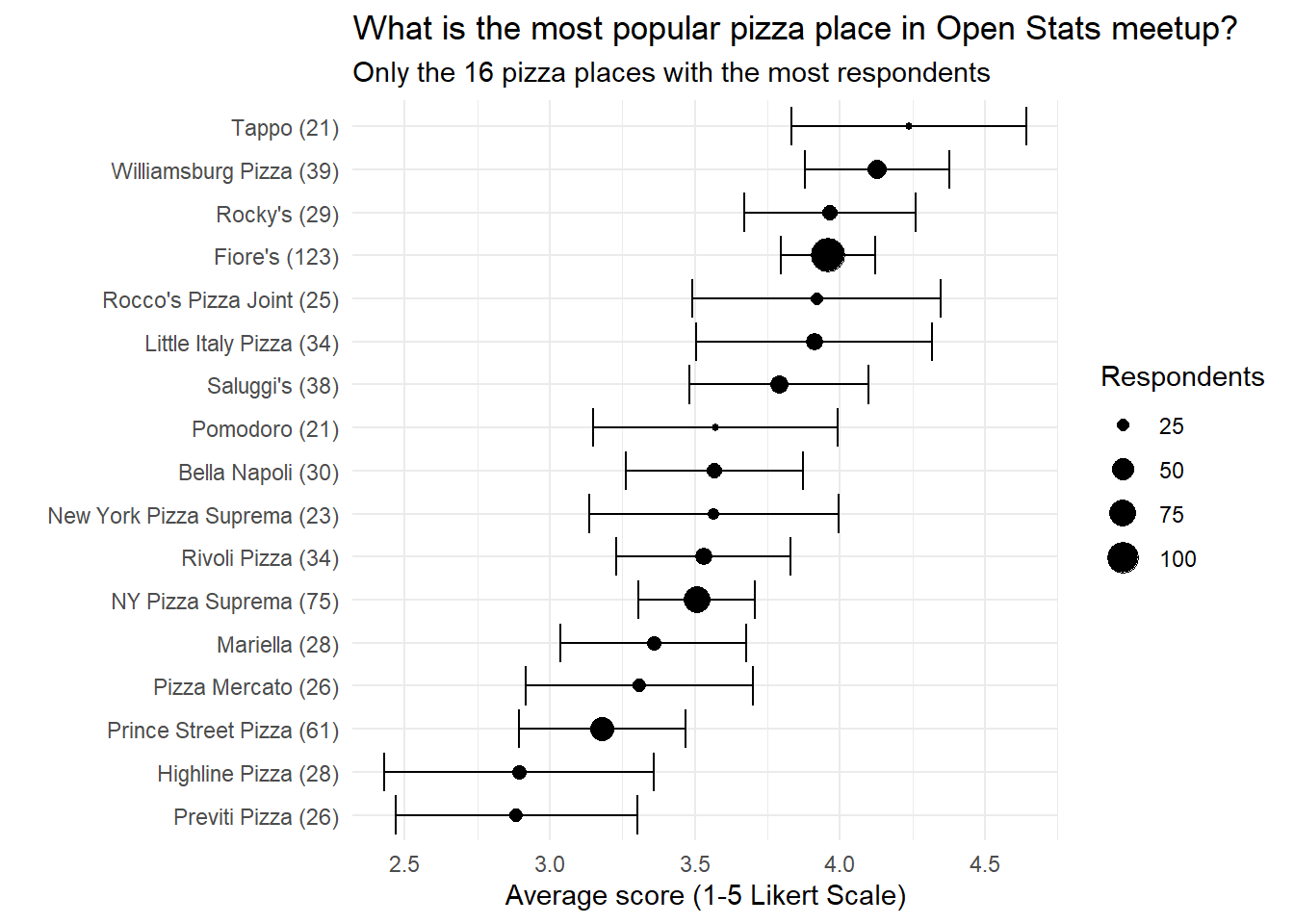
Where is the best places?
Now we’ll plot the evaluations of each place but also plot the confidence interval of each evaluation. First we build an auxiliary function to use with our dataset that sums each answer by place.
1
2
3
4
5
6
7
8
# generate a sample from 'x' with each 'frequency'# then apply a t.testt_test_repeated<-function(x,frequency){tidy(t.test(rep(x,frequency)))}# checkt_test_repeated(c(1,2,3,4,5),c(5,10,100,50,30))
1
2
3
4
## # A tibble: 1 x 8
## estimate statistic p.value parameter conf.low conf.high method alternative
## <dbl> <dbl> <dbl> <dbl> <dbl> <dbl> <chr> <chr>
## 1 3.46 53.5 4.45e-118 194 3.33 3.59 One Sam~ two.sided
# ploting the valuesby_place_answer%>%# pelo menos cinco votosfilter(total>=5)%>%# por localgroup_by(place,total)%>%# apply t.test in the answers# look that the column answer an votes, grouped by place, are "vectors"summarise(t_test_result=list(t_test_repeated(answer_integer,votes)))%>%ungroup()%>%unnest(t_test_result)%>%select(place,total,average=estimate,low=conf.low,high=conf.high)%>%mutate(place=glue("{place} ({total})"),# number of samplesplace=fct_reorder(place,average))%>%top_n(16,total)%>%ggplot(aes(average,place))+geom_point(aes(size=total))+geom_errorbarh(aes(xmin=low,xmax=high))+labs(x="Average score (1-5 Likert Scale)",y="",title="What is the most popular pizza place in Open Stats meetup?",subtitle="Only the 16 pizza places with the most respondents",size="Respondents")
# reading from githubpizza_barstool<-readr::read_csv("https://raw.githubusercontent.com/rfordatascience/tidytuesday/master/data/2019/2019-10-01/pizza_barstool.csv")pizza_barstool%>%glimpse()
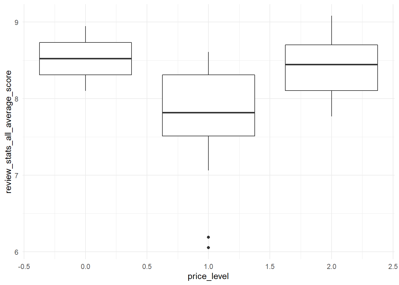
Do higher price place makes better evaluated pizzas?
1
2
3
4
5
6
# from places with more than 50 evaluationspizza_barstool%>%top_n(50,review_stats_all_count)%>%# plot price level vs reviewggplot(aes(price_level,review_stats_all_average_score,group=price_level))+geom_boxplot()
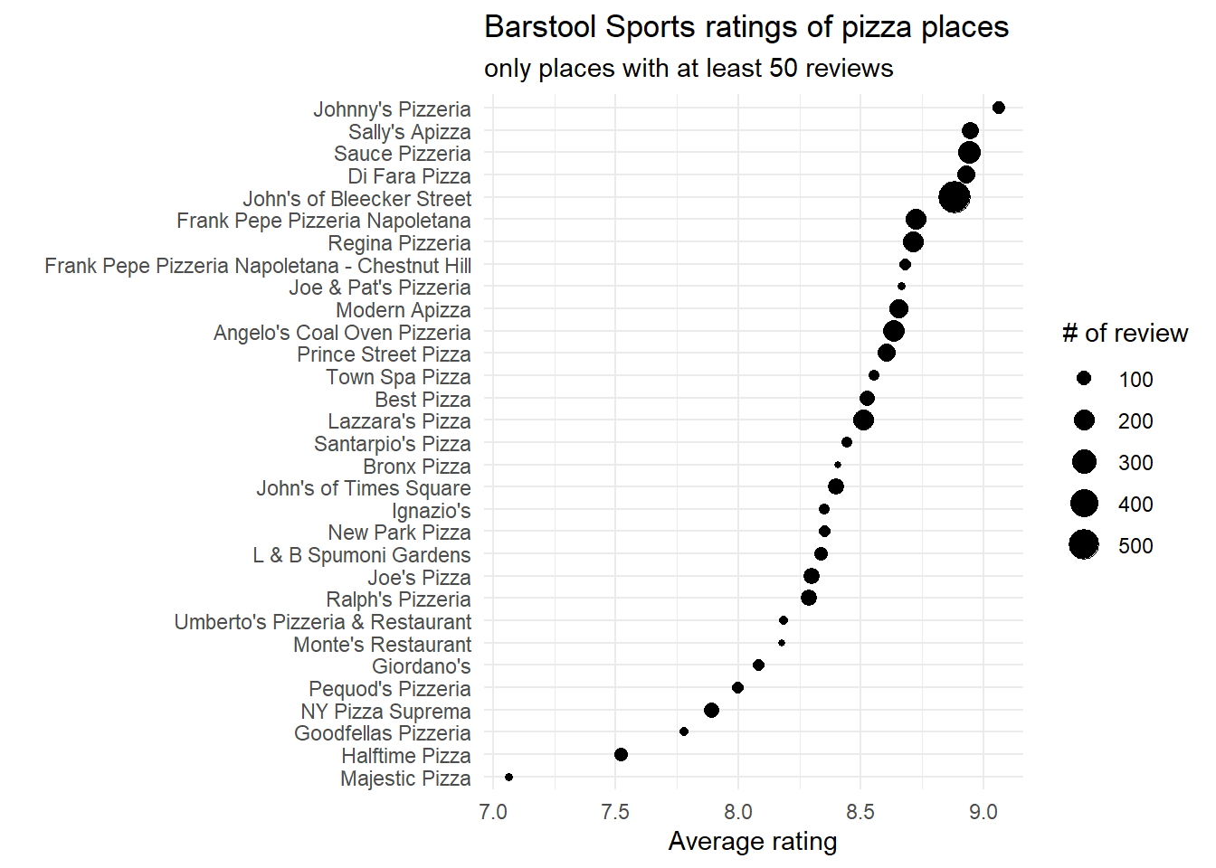
What are the places with best pizzas?
1
2
3
4
5
6
7
8
9
# from places with more than 50 evaluationspizza_barstool%>%filter(review_stats_all_count>=50)%>%mutate(name=fct_reorder(name,review_stats_all_average_score))%>%ggplot(aes(review_stats_all_average_score,name,size=review_stats_all_count))+geom_point()+labs(x="Average rating",size="# of review",y="",title="Barstool Sports ratings of pizza places",subtitle="only places with at least 50 reviews")
Where are these places?
1
2
3
4
5
6
7
8
9
10
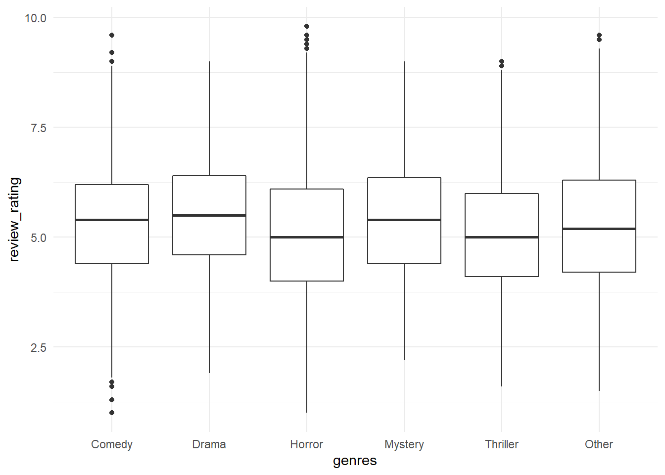
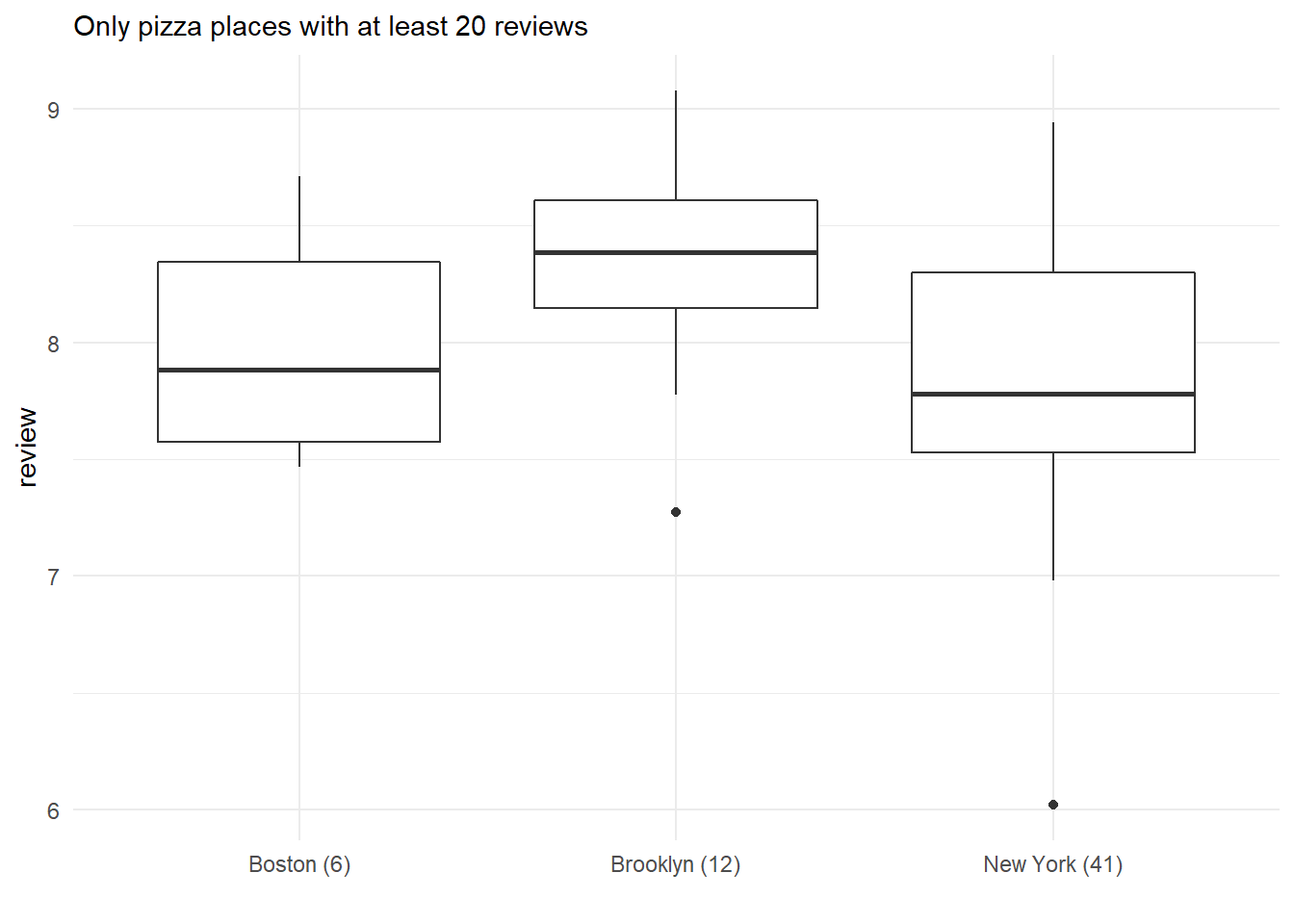
11
# What places have best pizzas?pizza_barstool%>%filter(review_stats_all_count>=20)%>%# by cityadd_count(city)%>%# cities with at least 6 placesfilter(n>=6)%>%mutate(city=glue("{city} ({n})"))%>%ggplot(aes(city,review_stats_all_average_score))+geom_boxplot()+labs(subtitle="Only pizza places with at least 20 reviews",y="review",x="")
Brooklyn has the best pizzas!
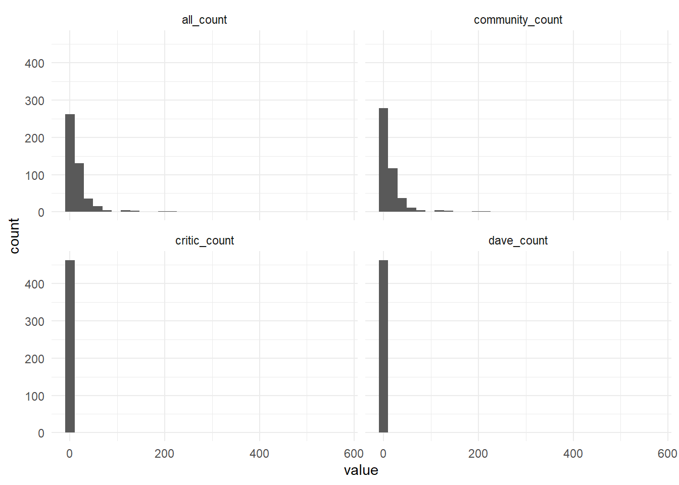
Comparing Reviews
The dataset has two kinds of pizza evaluation, let’s check the differences.
1
2
3
4
5
6
7
8
9
10
11
12
# select the reviewspizza_barstool%>%select(place=name,price_level,contains("review"))%>%rename_all(~str_remove(.,"review_stats_"))%>%select(-contains("provider"))%>%select(contains("count"))%>%gather(key,value)%>%ggplot(aes(value))+geom_histogram()+facet_wrap(~key)
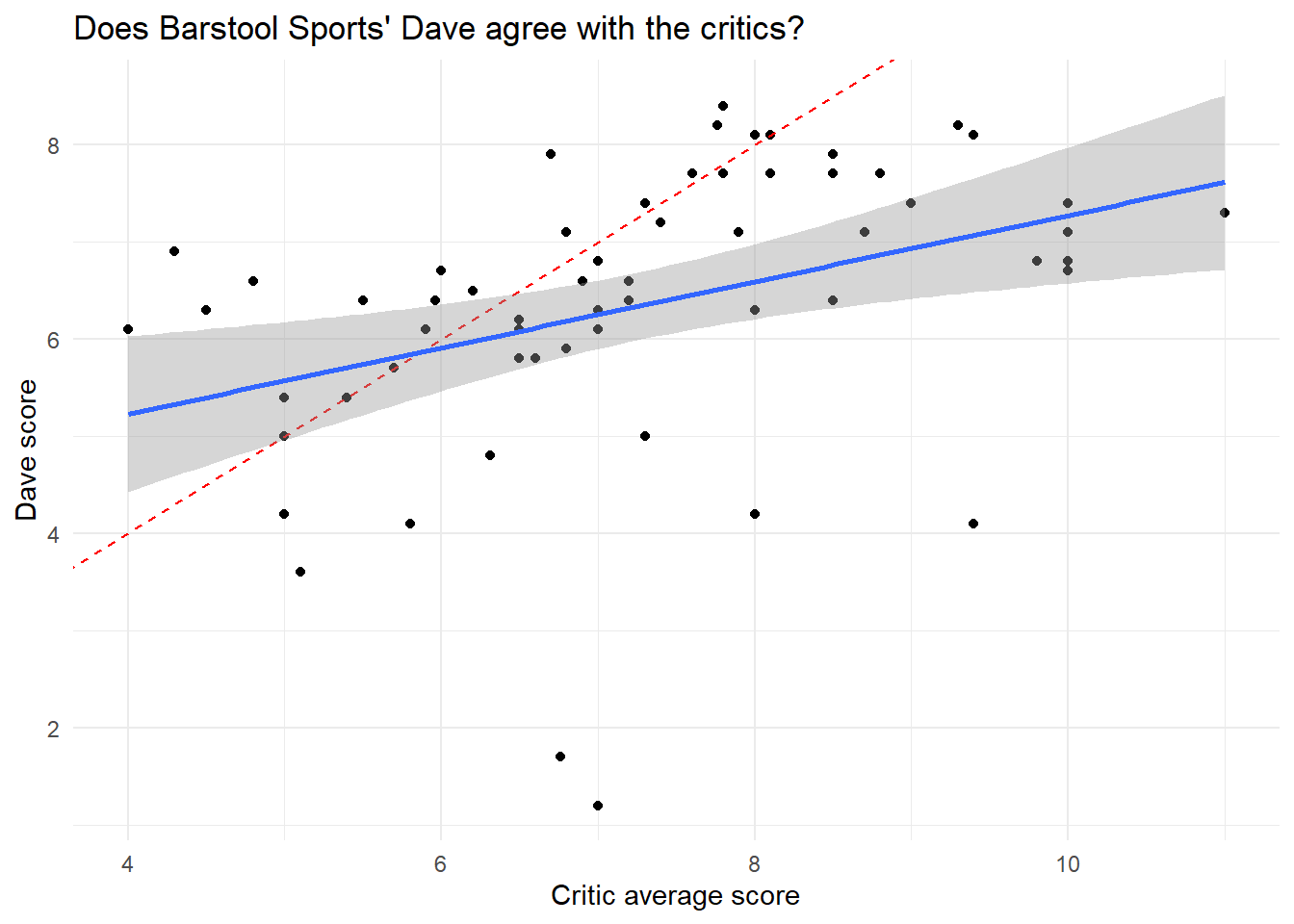
Does Barstool Sports' Dave agree with the critics?
 1
 2
 3
 4
 5
 6
 7
 8
 9
10
11
12
13
14
15
16
17
18
# taking the name, price and reviewspizza_cleaned<-pizza_barstool%>%select(place=name,price_level,contains("review"))%>%# cleaning column namesrename_all(~str_remove(.,"review_stats_"))%>%select(-contains("provider"))# ploting Daves x Criticspizza_cleaned%>%filter(critic_count>0)%>%ggplot(aes(critic_average_score,dave_average_score))+geom_point()+geom_abline(color="red",linetype="dashed")+# reference linegeom_smooth(method="lm")+labs(x="Critic average score",y="Dave score",title="Does Barstool Sports' Dave agree with the critics?")
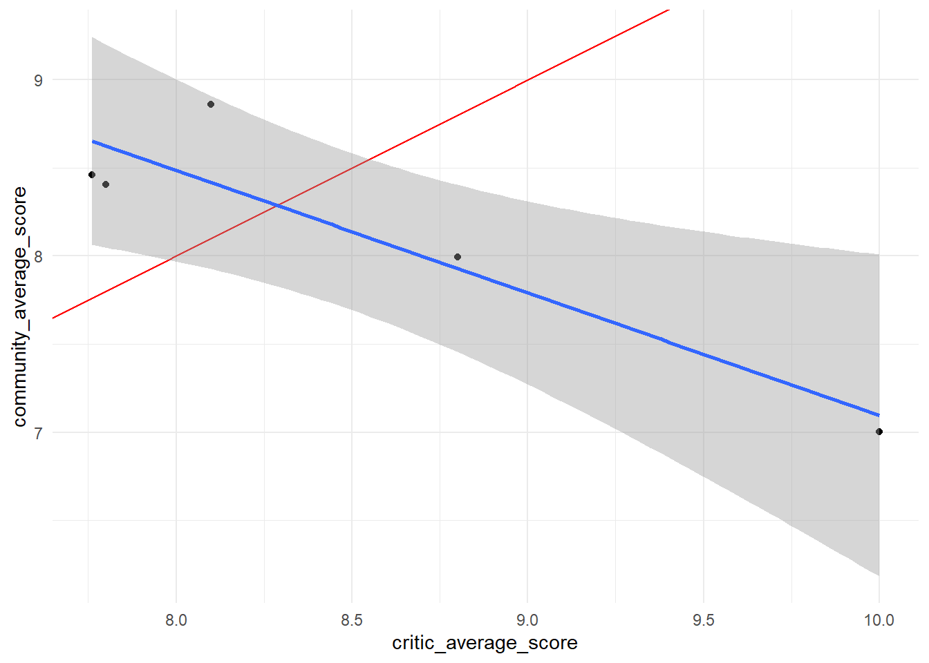
In overal the evaluations has some correlation. Let’s see Community vs Critics
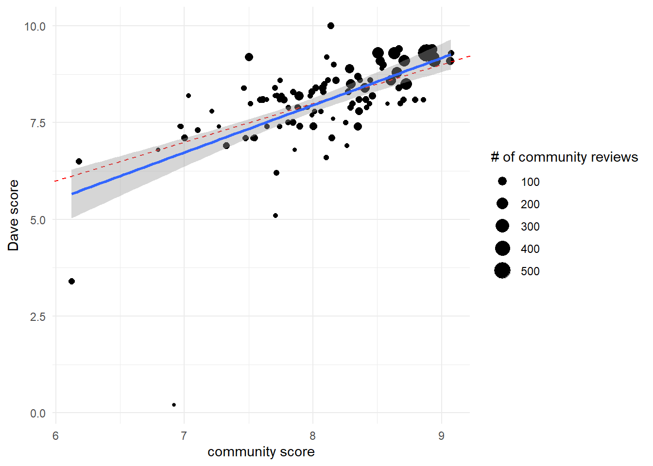
pizza_cleaned%>%filter(community_count>=20)%>%ggplot(aes(community_average_score,dave_average_score))+geom_point(aes(size=community_count))+geom_abline(color="red",linetype="dashed")+geom_smooth(method="lm")+labs(size="# of community reviews",x="community score",y="Dave score")
Dave score are remarkable close to the community reviews.