I’ll start series of posts about Keras, a high-level neural networks API developed with a focus on enabling fast experimentation, running on top of TensorFlow, but using its R interface. To start, we’ll review our LeNet implemantation with MXNET for MNIST problem, a traditional “Hello World” in the Neural Network world.
About Keras in R
Keras is an API for building neural networks written in Python capable of running on top of Tensorflow, CNTK, or Theano. It was developed with a focus on enabling fast experimentation. Being able to go from idea to result with the least possible delay is key to doing good research.
We’ll use a R implementation of Keras, that communicates with the Python environment using the Reticulate Package to build and run neural networks on Tensorflow back end.
Instruction for Setup
It’s necessary to install Python and Tensorflow environments in your machine, also, to do the Tensorflow run over a GPU you will need install NVIDIA’s CUDA Toolkit and cuDNN libraries. In my experience, this is very easy and cheap using an Ubuntu preemptible Google Compute Engine instance. You can follow one of the setup instructions here:
Dataset and Tensors
The Keras package already provides some datasets and pre-trained networks to serve as a learning base, the MNIST dataset is one of them, let’s use it.
 1
 2
 3
 4
 5
 6
 7
 8
 9
10
11
12
13
14
|
# loading keras lib
library(keras)

# loading and preparing dataset
mnist <- dataset_mnist()

# separate the datasets
x.train <- mnist$train$x
lbl.train <- mnist$train$y
x.test <-  mnist$test$x
lbl.test <-  mnist$test$y

# let's see what we have
str(x.train)
|
1
|
## int [1:60000, 1:28, 1:28] 0 0 0 0 0 0 0 0 0 0 ...
|
1
|
## int [1:60000(1d)] 5 0 4 1 9 2 1 3 1 4 ...
|
1
2
|
##    Min. 1st Qu.  Median    Mean 3rd Qu.    Max.
##    0.00    0.00    0.00   33.32    0.00  255.00
|
The first time you invoke dataset_mnist() the data will be downloaded. We can see that we get in reply a three-dimensional array, in the first dimension we have the index of the case, and for each one of them, we have a matrix of 28x28 that corresponds to a image of a number.
To use with “tensorflow/keras” it is necessary to convert the matrix into a Tensor (generalization of a vector), in this case we have to convert to 4D-Tensor, with dimensions of “n x 28 x 28 x 1”, where:
- “n” is the “case number”
- “28 x 28” are the width and height of the image, and
- “1” is the “channel” (or “value”), for each pixel of the image
The channel in the image stands for the “color encoding”. In color images, usually the channel will be a 3-dimensional vector, for RGB values. In the MNIST database, the images are im grey scale, in integers from 0 to 255. To work with neural networks is advisable to normalize it into to a float value, from 0.0 to 1.0. to do that we simple divide the values by 255.
1
2
3
4
5
6
7
8
9
|
# Redefine dimension of train/test inputs to 2D "tensors" (28x28x1)
x.train <- array_reshape(x.train, c(nrow(x.train), 28,28,1))
x.test  <- array_reshape(x.test,  c(nrow(x.test),  28,28,1))

# normalize values to be between 0.0 - 1.0
x.train <- x.train/255
x.test  <- x.test/255

str(x.train)
|
1
|
## num [1:60000, 1:28, 1:28, 1] 0 0 0 0 0 0 0 0 0 0 ...
|
1
2
|
##    Min. 1st Qu.  Median    Mean 3rd Qu.    Max.
##  0.0000  0.0000  0.0000  0.1307  0.0000  1.0000
|
In addition, it is necessary to convert the classification labels using one-hot encoding, since we neural network classifies the image into one of the ten possibilities (from 0 to 9).
1
2
3
4
5
|
# one hot encoding
y.train <- to_categorical(lbl.train,10)
y.test  <- to_categorical(lbl.test,10)

str(y.train)
|
1
|
## num [1:60000, 1:10] 0 1 0 0 0 0 0 0 0 0 ...
|
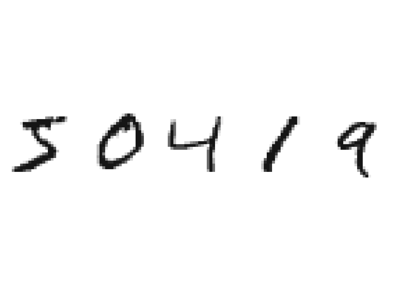
Let’s visualize some numbers in the dataset.
 1
 2
 3
 4
 5
 6
 7
 8
 9
10
11
|
# plot one case
show_digit <- function(tensor, col=gray(12:1/12), ...) {
  tensor %>%
    apply(., 2, rev) %>%      # reorient to make a 90 cw rotation
    t() %>%                   # reorient to make a 90 cw rotation
    image(col=col, axes=F, asp=1, ...)       # plot matrix as image
}

# check some data
par(mfrow=c(1,5), mar=c(0.1,0.1,0.1,0.1))
for(i in 1:5) show_digit(x.train[i,,,])
|

LeNet Architecture
I’ll use one of the LeNet architecture for the neural network, based in two sets of Convolutional filters and pooling for the convolutional layers and then two fully connected layers as classification group, as show bellow:

In Keras, we’ll build a sequential model, adding layer by layer in the network.
 1
 2
 3
 4
 5
 6
 7
 8
 9
10
11
12
13
14
|
# build lenet
keras_model_sequential() %>%
  layer_conv_2d(input_shape=c(28,28,1), filters=20, kernel_size = c(5,5), activation = "tanh") %>%
  layer_max_pooling_2d(pool_size = c(2,2), strides = c(2,2)) %>%
  layer_conv_2d(filters = 50, kernel_size = c(5,5), activation="tanh" ) %>%
  layer_max_pooling_2d(pool_size = c(2,2), strides = c(2,2) ) %>%
  layer_dropout(rate=0.3) %>%
  layer_flatten() %>%
  layer_dense(units = 500, activation = "tanh" ) %>%
  layer_dropout(rate=0.3) %>%
  layer_dense(units=10, activation = "softmax") -> model

# lets look the summary
summary(model)
|
 1
 2
 3
 4
 5
 6
 7
 8
 9
10
11
12
13
14
15
16
17
18
19
20
21
22
23
24
25
26
27
|
## Model: "sequential"
## ________________________________________________________________________________
##  Layer (type)                       Output Shape                    Param #
## ================================================================================
##  conv2d_1 (Conv2D)                  (None, 24, 24, 20)              520
##
##  max_pooling2d_1 (MaxPooling2D)     (None, 12, 12, 20)              0
##
##  conv2d (Conv2D)                    (None, 8, 8, 50)                25050
##
##  max_pooling2d (MaxPooling2D)       (None, 4, 4, 50)                0
##
##  dropout_1 (Dropout)                (None, 4, 4, 50)                0
##
##  flatten (Flatten)                  (None, 800)                     0
##
##  dense_1 (Dense)                    (None, 500)                     400500
##
##  dropout (Dropout)                  (None, 500)                     0
##
##  dense (Dense)                      (None, 10)                      5010
##
## ================================================================================
## Total params: 431,080
## Trainable params: 431,080
## Non-trainable params: 0
## ________________________________________________________________________________
|
Also, we have to define some “learning parameters” for our network using compile() function, they are:
- Loss function: a method of evaluating how well your algorithm models your dataset.
- Optimizer/Learning Rate: together the loss function and model parameters by updating the model in response to the output of the loss function
- Evaluation Metrics: influences how the performance of machine learning algorithms is measured and compared
1
2
3
4
5
6
|
# keras compile
model %>% compile(
  loss = "categorical_crossentropy",
  optimizer = optimizer_rmsprop(),
  metrics = c('accuracy')
)
|
Train and Evaluate
Finally, your network is ready to train, let’s to it with fit() function.
1
2
3
4
5
6
7
8
|
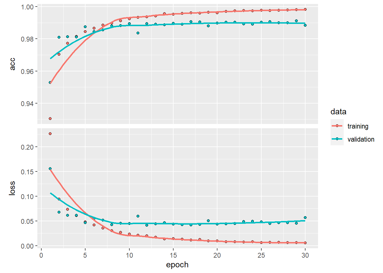
# train the model and store the evolution history
history <- model %>% fit(
  x.train, y.train, epochs=30, batch_size=128,
  validation_split=0.3
)

# plot the network evolution
plot(history)
|

Let’s see how good the fitted model are applying the model in the test set
1
2
|
# evaluating the model
evaluate(model, x.test, y.test)
|
1
2
|
##       loss   accuracy
## 0.04707442 0.99000001
|
As you see, it’s an impressive 99% of accuracy.
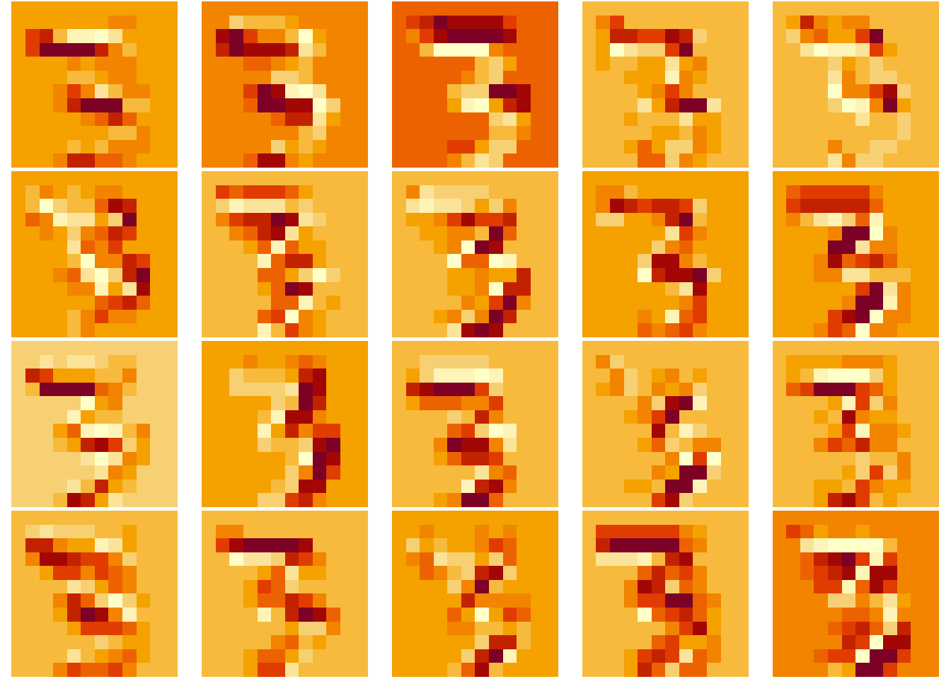
Visualizing the Activation Layers
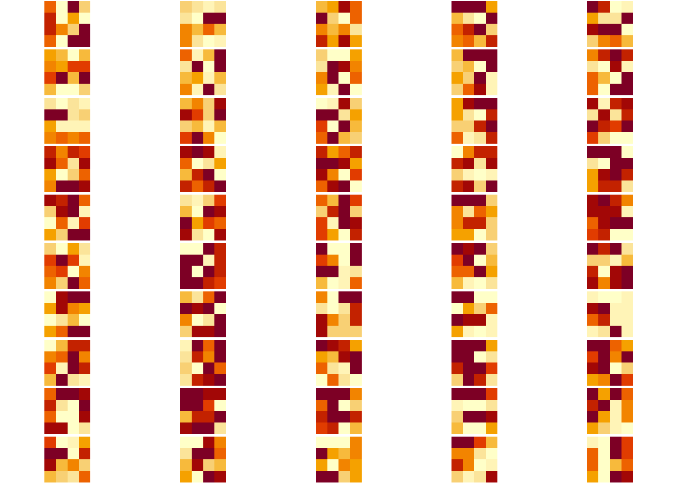
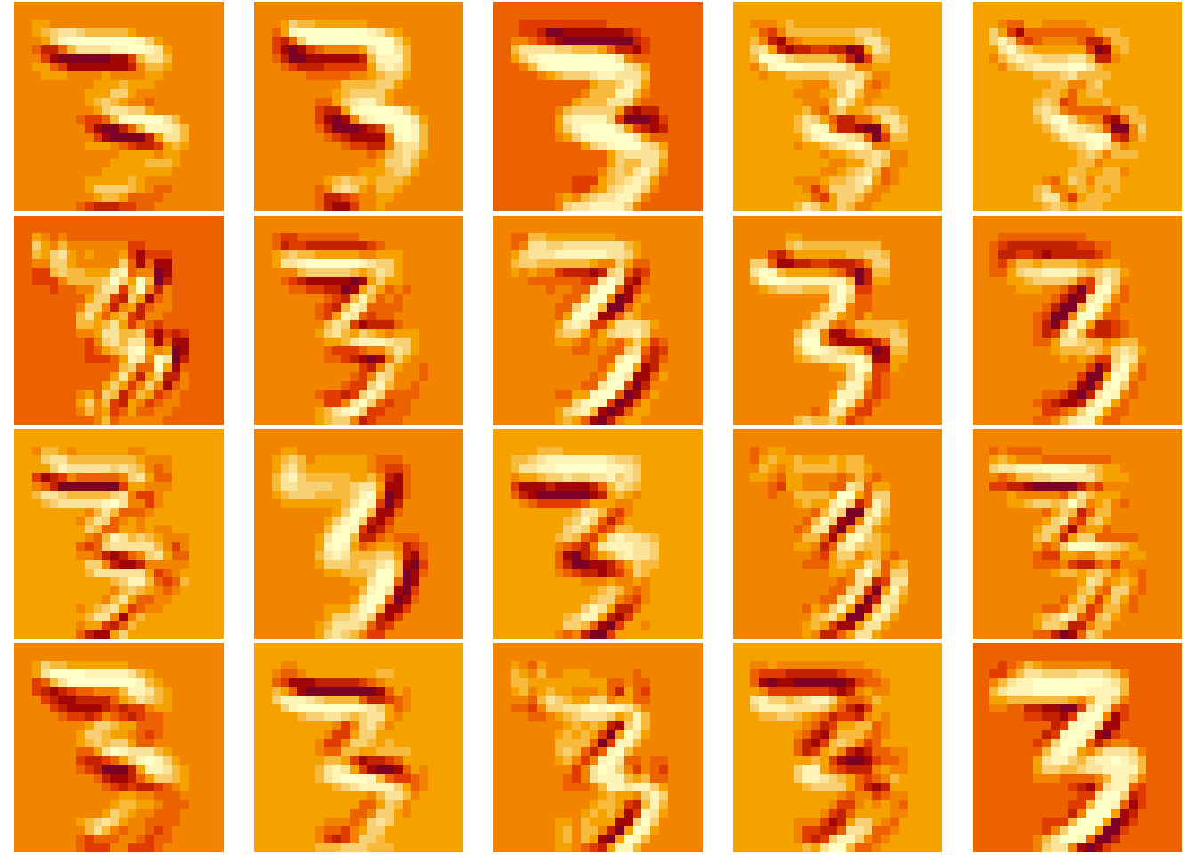
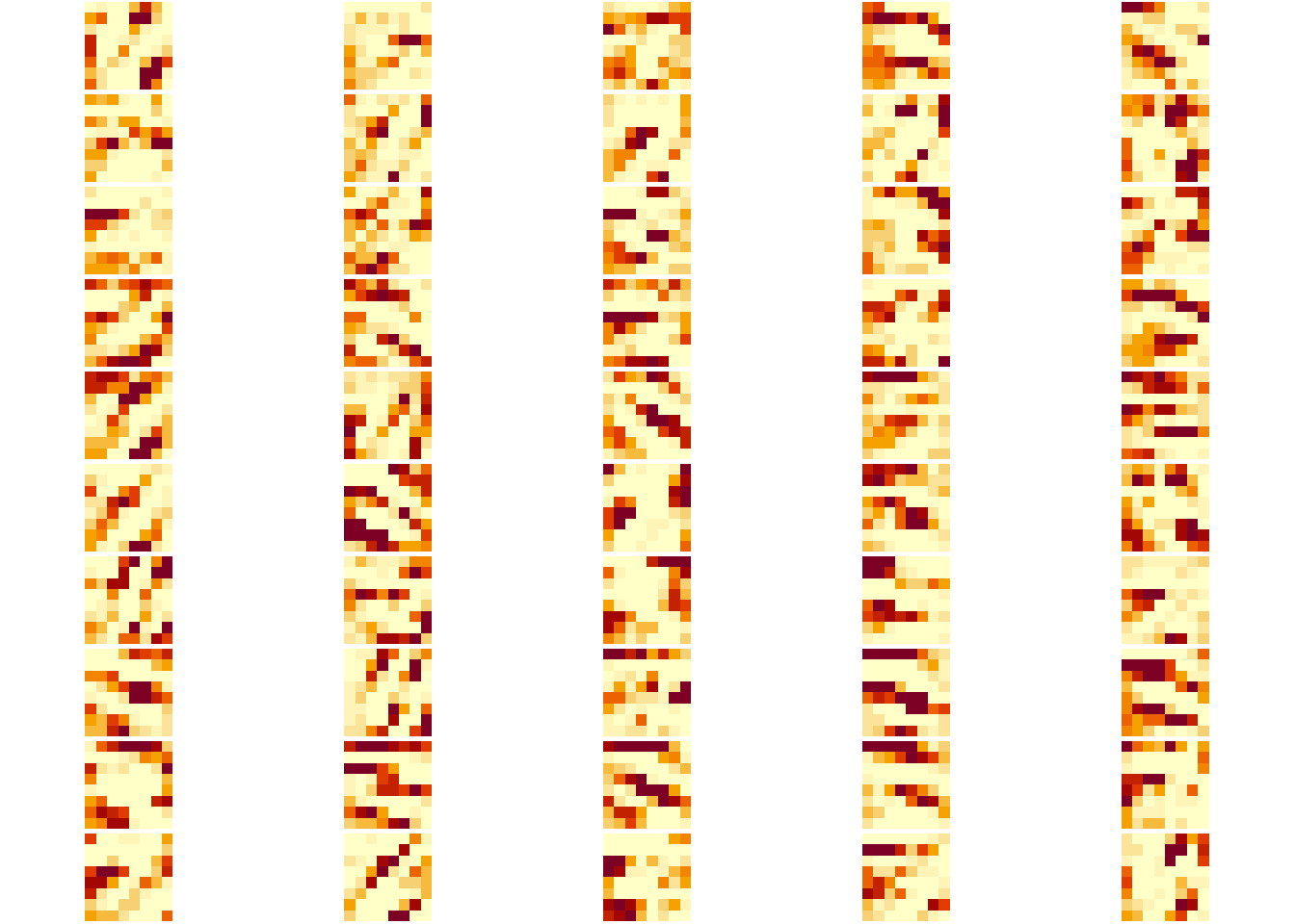
As we did in the mxnet post, let’s see how the internal layers react to a input data, visualizing the neuron’s activations pattern in the conv layers:
 1
 2
 3
 4
 5
 6
 7
 8
 9
10
11
12
13
14
15
16
17
18
19
20
21
22
23
24
25
26
27
|
# Extracts the outputs of the top 8 layers:
layer_outputs <- lapply(model$layers[1:8], function(layer) layer$output)

# Creates a model that will return these outputs, given the model input:
activation_model <- keras_model(inputs = model$input, outputs = layer_outputs)

# choose a case
a_digit <- array_reshape(x.train[45,,,], c(1,28,28,1))

# Returns a list of five arrays: one array per layer activation
activations <- activation_model %>% predict(a_digit)

# plot a tensor channel
plot_channel <- function(channel) {
  rotate <- function(x) t(apply(x, 2, rev))
  image(rotate(channel), axes = FALSE, asp = 1)
}

# plot the channels of a layout ouput (activation)
plotActivations <- function(.activations, .index){
  layer_inpected <- .activations[[.index]]
  par(mfrow=c(dim(layer_inpected)[4]/5,5), mar=c(0.1,0.1,0.1,0.1))
  for(i in 1:dim(layer_inpected)[4]) plot_channel(layer_inpected[1,,,i])
}

# look the 2D layers activations
plotActivations(activations, 1) # conv2D - tanh
|

1
|
plotActivations(activations, 2) # max pooling
|

1
|
plotActivations(activations, 3) # conv2D - tanh
|

1
|
plotActivations(activations, 4) # max pooling
|
