kNN Analysis on MNIST with 97% accuracy

Usually Yann LeCun’s MNIST database is used to explore Artificial Neural Network architectures for image recognition problem.
In the last post the use of a ANN (LeNet architecture) implemented using mxnet to resolve this classification problem.
But in this post, we’ll see that the MNIST problem isn’t a difficult one, only resolved by ANNs, analyzing the data set we can see that is possible, with a high degree of precision, resolving this classification problem with a simple k-nearest neighbors algorithm.
setup
library(tidyverse)  # for plot and data manipulation
library(factoextra) # to plot PCA values
library(plotly)     # 3D interactive plots
library(class)      # KNN algorithm
library(caret)      # Near Zero Var removing
MNist Dataset
Download all four data set files from MNIST site and gunzip them in the project directory.
The default MNIST data set is somewhat inconveniently formatted, but we use an adaptation of gist from Brendan o’Connor to read the files transforming them in a structure simple to use and access.
### load database

# read function returns a list of datasets
load_mnist <- function() {
  load_image_file <- function(filename) {
    ret = list()
    f = file(filename,'rb')
    readBin(f,'integer',n=1,size=4,endian='big')
    ret$n = readBin(f,'integer',n=1,size=4,endian='big')
    nrow = readBin(f,'integer',n=1,size=4,endian='big')
    ncol = readBin(f,'integer',n=1,size=4,endian='big')
    x = readBin(f,'integer',n=ret$n*nrow*ncol,size=1,signed=F)
    ret$x = matrix(x, ncol=nrow*ncol, byrow=T)
    close(f)
    ret
  }
  load_label_file <- function(filename) {
    f = file(filename,'rb')
    readBin(f,'integer',n=1,size=4,endian='big')
    n = readBin(f,'integer',n=1,size=4,endian='big')
    y = readBin(f,'integer',n=n,size=1,signed=F)
    close(f)
    y
  }
  train <- load_image_file('./data/train-images.idx3-ubyte')
  test <- load_image_file('./data/t10k-images.idx3-ubyte')

  train$y <- load_label_file('./data/train-labels.idx1-ubyte')
  test$y <- load_label_file('./data/t10k-labels.idx1-ubyte')

  return(
    list(
      train = train,
      test = test
    )
  )
}

# load in 'mnist' var
mnist <- load_mnist()

# look the data format
str(mnist)

## List of 2
##  $ train:List of 3
##   ..$ n: int 60000
##   ..$ x: int [1:60000, 1:784] 0 0 0 0 0 0 0 0 0 0 ...
##   ..$ y: int [1:60000] 5 0 4 1 9 2 1 3 1 4 ...
##  $ test :List of 3
##   ..$ n: int 10000
##   ..$ x: int [1:10000, 1:784] 0 0 0 0 0 0 0 0 0 0 ...
##   ..$ y: int [1:10000] 7 2 1 0 4 1 4 9 5 9 ...
The gist read the binary MNIST files and returns a convenient list for training cases and test cases, each with size (n), the pixels (x) and the labels (y).
Let’s see some of the images represented in the x variable.
# functino plot one case digit (by 1d array of 784 pixels)
show_digit <- function(arr784, col=gray(25:1/25), ...) {
  image(matrix(arr784, nrow=28)[,28:1], col=col, ...)
}

# showing first 25 cases
labels <- paste(mnist$train$y[1:25],collapse = ", ")
par(mfrow=c(5,5), mar=c(0.1,0.1,0.1,0.1))
for(i in 1:25) show_digit(mnist$train$x[i,], axes=F)
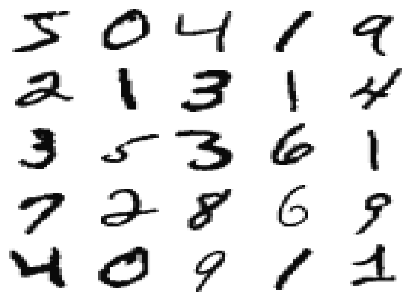
Each line in x var is a digit case, and each column represents the intensity of a pixel in a 28 x 28 image.
Data Analysis
How the each pixels in the image behavior in the “average” for each digit? It’s possible to use this information to classify an digit?
Centroid
# calc digits centroids
centroids <- list()
for(i in 0:9) {
  x <- mnist$train$x[(mnist$train$y == i),]
  centroids[[i+1]] <- colMeans(x)
}

# ploting the centroids
par(mfrow=c(2,5), mar=c(0.1,0.1,0.1,0.1))
res <- lapply(X = centroids, show_digit, xaxt='n', yaxt='n')
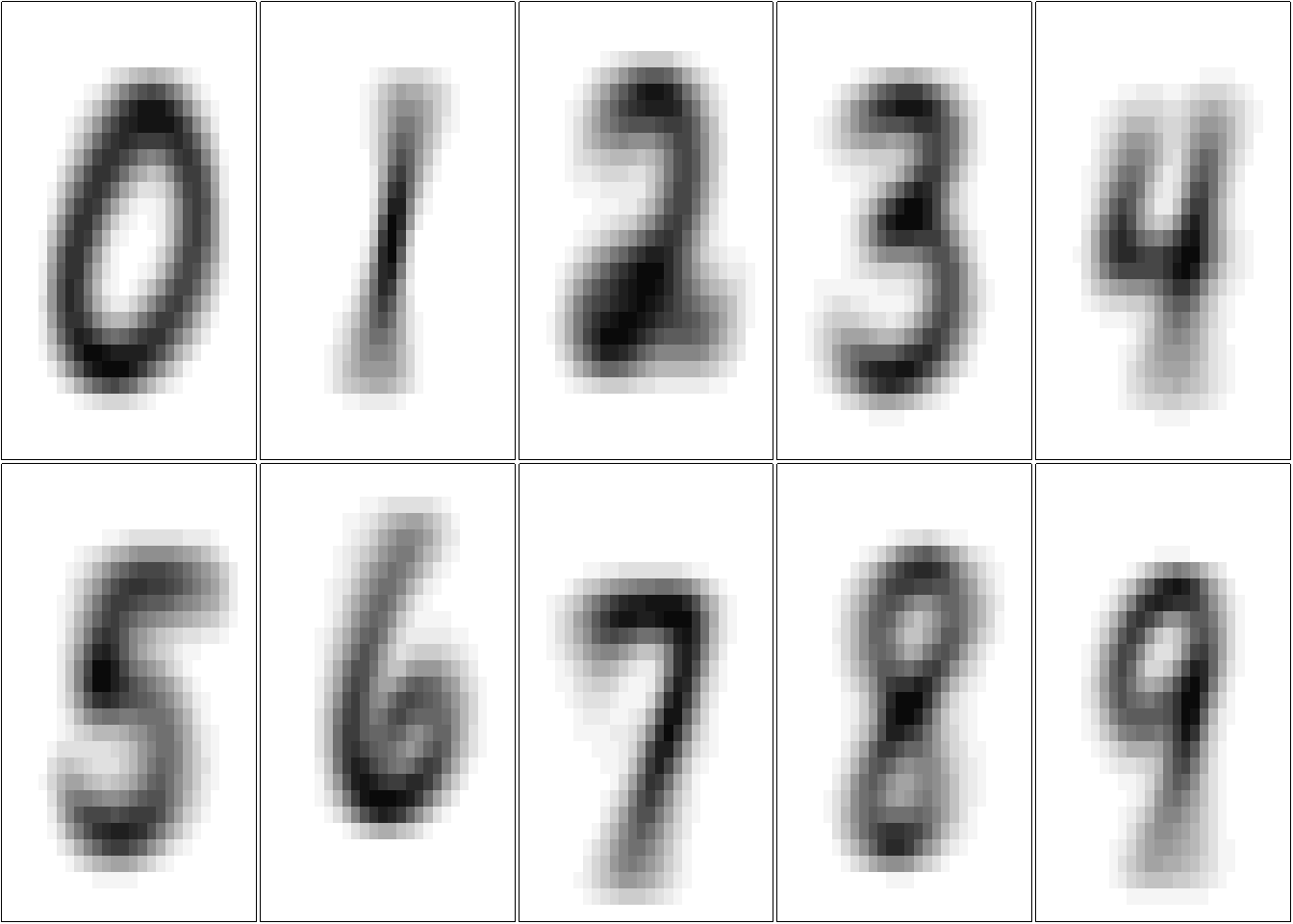
These averaged images are called centroids. We’re treating each image as a 784-dimensional point (28 by 28), and then taking the average of all points in each dimension individually.
We see that each centroid has a good representation of a digit, so each image in the data set are centralized in the image and there is not large variations. Maybe we can use one elementary machine learning method: nearest centroid classifier, would ask for each image which of these centroids it comes closest to.1
Compare Centroids
How different one centroid is from other? We can simply take the difference between the pixel values for each digit pair like this:
# compare cases
compare <- tidyr::crossing(comp1 = 0:9, comp2 = 0:9)

# calc features differences between the centroids
res <- apply(compare, 1, function(x,m=centroids){
  unlist(m[x[1]+1]) - unlist(m[x[2]+1])
}) %>% t() %>% as_tibble()

centroids_diff <- bind_cols(compare, res)

# plot them
par(mfrow=c(10,10), mar=c(0,0,0,0))
colFunc <- colorRampPalette(c("red","white","blue"))
res <- sapply(1:100, FUN=function(x) show_digit(as.matrix(centroids_diff[x,3:786]),
                                                col=colFunc(35),
                                                axes=F))
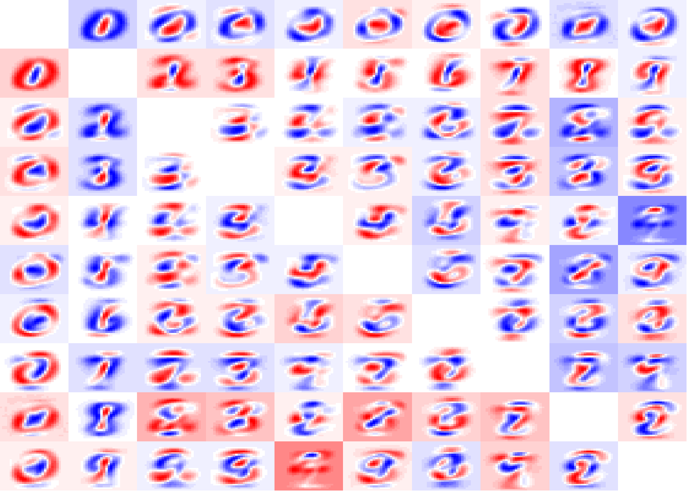
From the image we can see some “patterns” emerging from this. As higher are stains in this image more separable a digit from another is. We look particularly for 0 and 1 digits are strongly separable. But in fade images we have a problem, because the pixels are not ‘that’ different from one digit from other, like 4 x 9 and 3 x 8.
Distance
We can “measure” this difference, taking each pixel as a dimensions in the digit represent space and apply a simple euclidian distance between these data.
# calculating the distance between the centroids in 786 dimensions
dist <- apply(compare,1,function(x,m=centroids){
  sqrt(mean((unlist(m[x[1]+1])-unlist(m[x[2]+1]))^2))
}) %>% as_tibble()
centroids_dist <- bind_cols(compare,dist)

# ploting the distances
ggplot(centroids_dist, aes(x=comp1, y=comp2, fill=value)) +
  geom_tile() +
  geom_text(aes(label=round(value))) +
  scale_fill_gradient2(low = "blue", high = "red") +
  scale_x_continuous(breaks=0:9) +
  scale_y_continuous(breaks=0:9) +
  ylab("") + xlab("") +
  theme_bw()
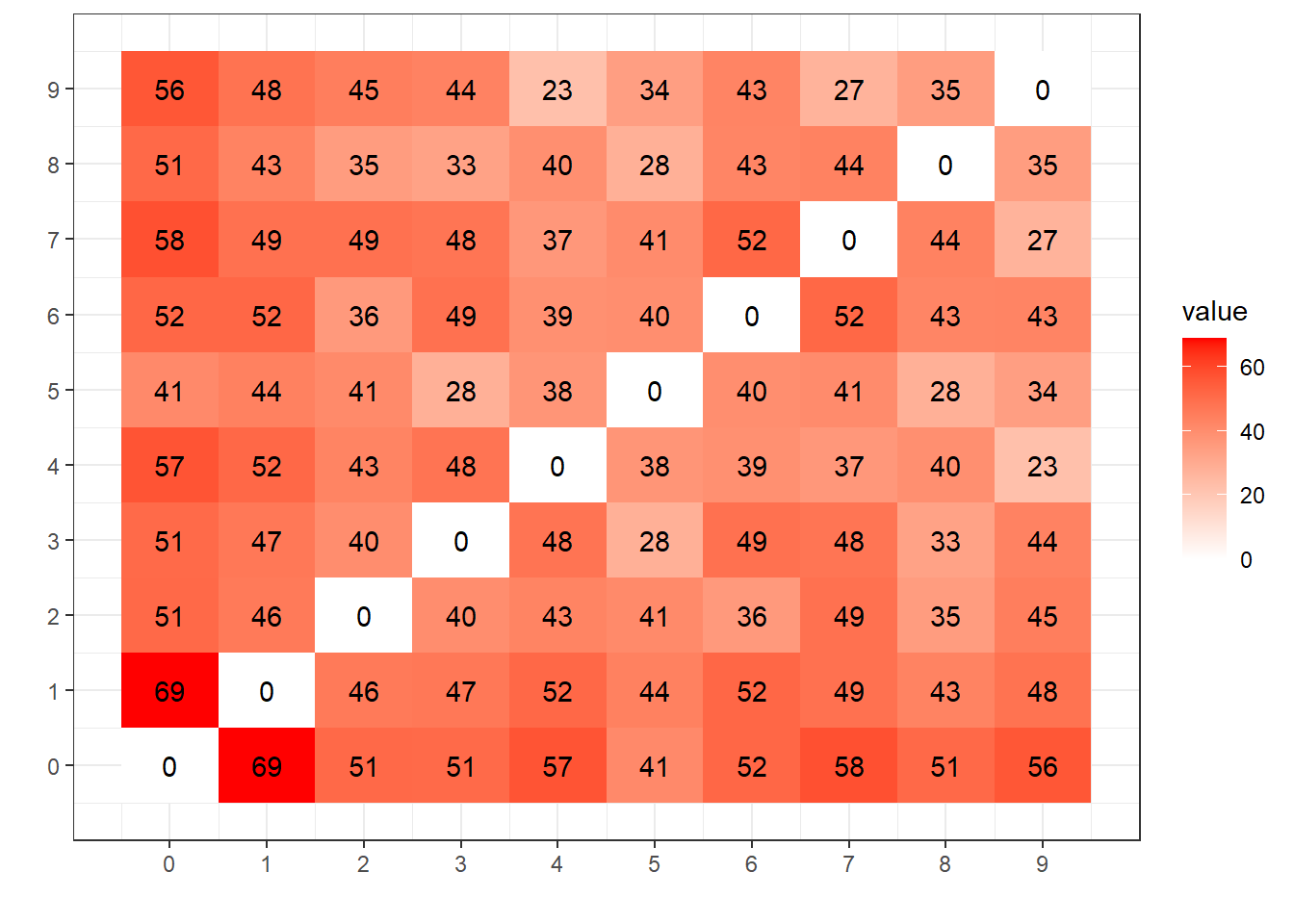
The distance here, measures the degree of “difference” between the centroids, and this matrix bring us a coll view, look at 0x1 how distance they are (69), making them easier to classify. Look at 4x9, they are more next (23), let’s compare this with the confusion matrix generated by the LeNet ANN from the last post:
##           Reference
## Prediction    0    1    2    3    4    5    6    7    8    9
##          0  974    0    1    0    0    2    3    0    2    0
##          1    1 1131    0    0    0    0    2    2    0    0
##          2    0    0 1025    1    1    0    0    2    0    0
##          3    0    0    0 1000    0    5    1    1    1    2
##          4    0    0    1    0  970    0    0    1    0    6
##          5    1    0    0    6    0  878    4    0    2    2
##          6    3    2    1    0    1    2  947    0    0    1
##          7    1    0    2    0    0    0    0 1016    0    3
##          8    0    2    2    3    0    4    1    1  966    1
##          9    0    0    0    0   10    1    0    5    3  994
We see the 16 mismatches involving cases 4x9, the largest.
Principal Component Analysis
We can improve this, it’s not all the pixels that have the same importance in the digit differentiation, some pixels (in the image borders, for example) don’t change its value along the data set and some pixels change very few from one digit to other. We transform the data sets to evidence the first removing the zero variance pixels and the second using Principal component Analysis or PCA.
# transforming in a matrix
tr.x <- mnist$train$x
ts.x <- mnist$test$x
all.x <- rbind(tr.x,ts.x)

# calculating the PCA

# removing zero or near zero variance features
nzv <- nearZeroVar(all.x, saveMetrics = T)
all.x <- all.x[,!nzv$zeroVar]

# principal component analysis
pca <- prcomp(all.x, center = T)
saveRDS(pca, "pca.rds") # store to save time in the future
print(paste0("Columns with zero variance: ", sum(nzv$zeroVar)))

## [1] "Columns with zero variance: 65"
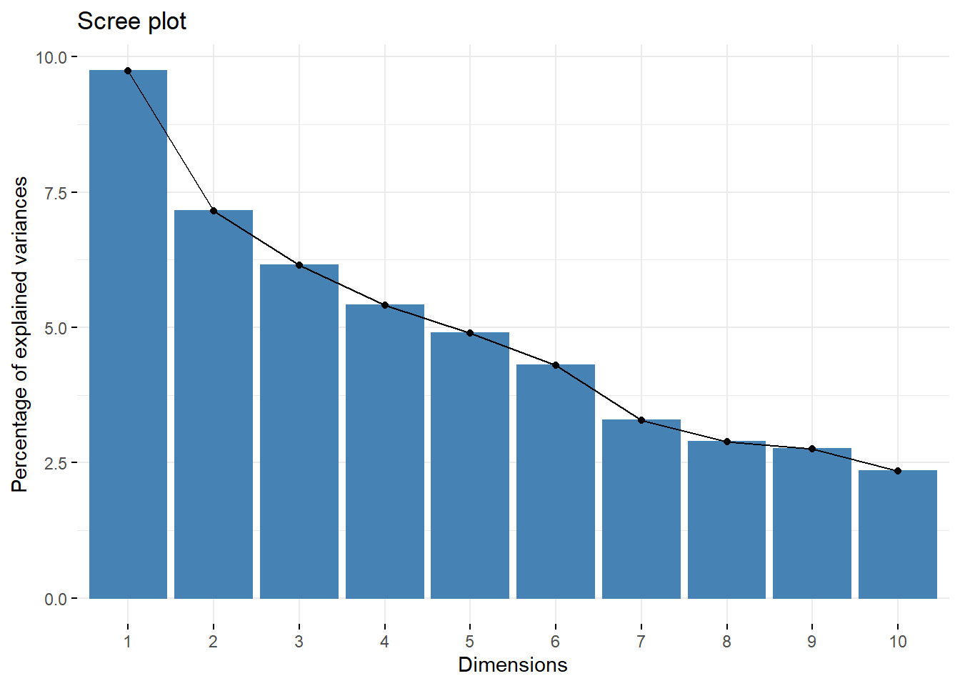
Principal Componets
This is the classic view of the first 10 principal components, they explain 49% of total variance of data set.
# principals component
fviz_eig(pca)
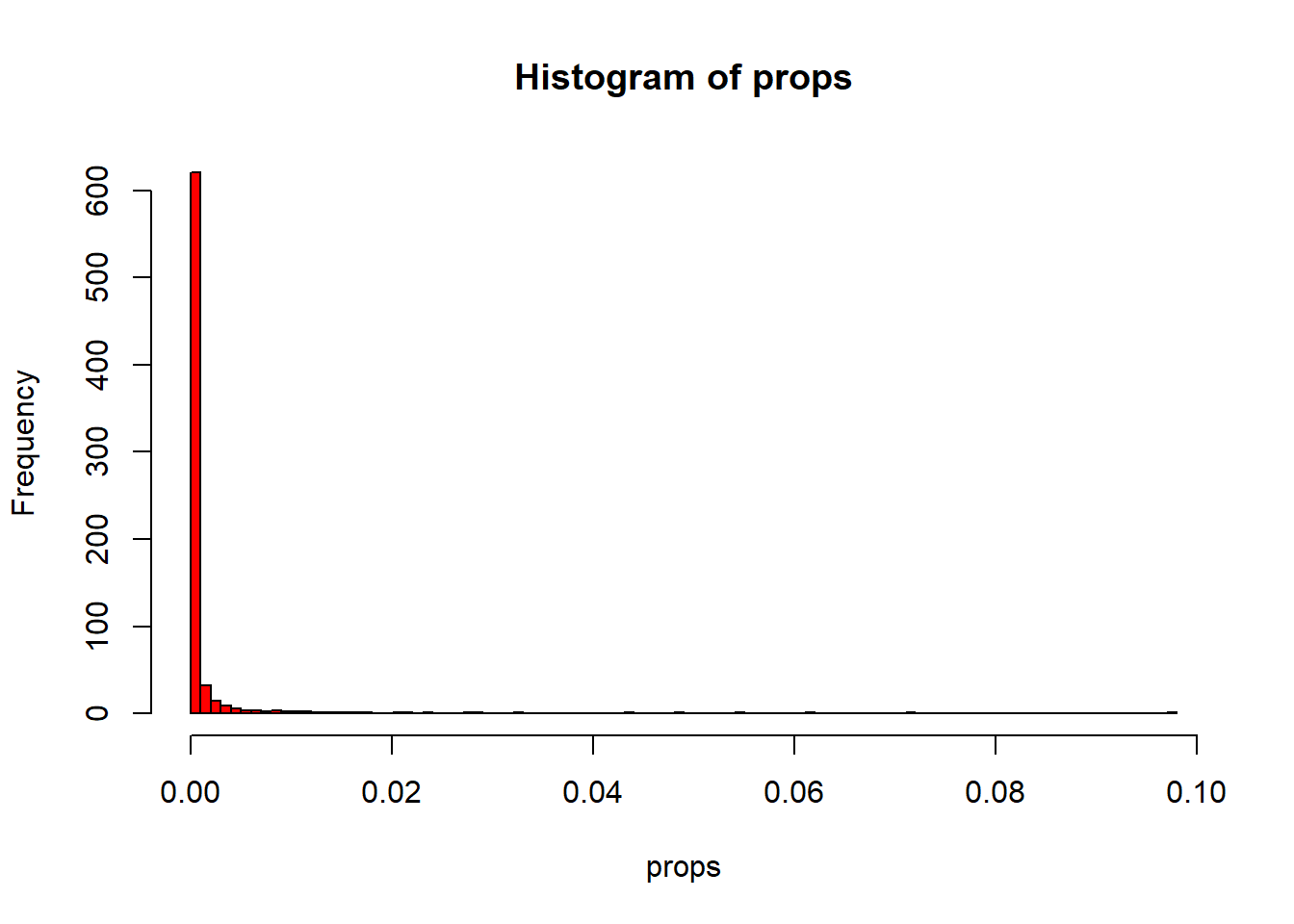
Distribution of variance
Indeed, we see that the majority of the dimensions has near zero variance and few pixels explain a lot.
# rebuilding features (transformed)
tr.x <- pca$x[(1:mnist$train$n),]
ts.x <- pca$x[(mnist$train$n+1):(mnist$train$n+mnist$test$n),]

vars <- apply(pca$x, 2, var)
props <- vars / sum(vars)

# distribuicao da % de sdev por
# res <- dev.off() # reset plot parameters
hist(props, breaks = 100, col="Red")
Cumulative Variance
Let’s see how much dimension of the PCA we need to consider.
# ploting the cumulative variance
data_frame(x=1:length(pca$sdev), sdev.cum=cumsum(props)) %>%
  ggplot(aes(x=x, y=sdev.cum)) +
  geom_line(color="darkblue", size=.8) +
  theme_minimal()
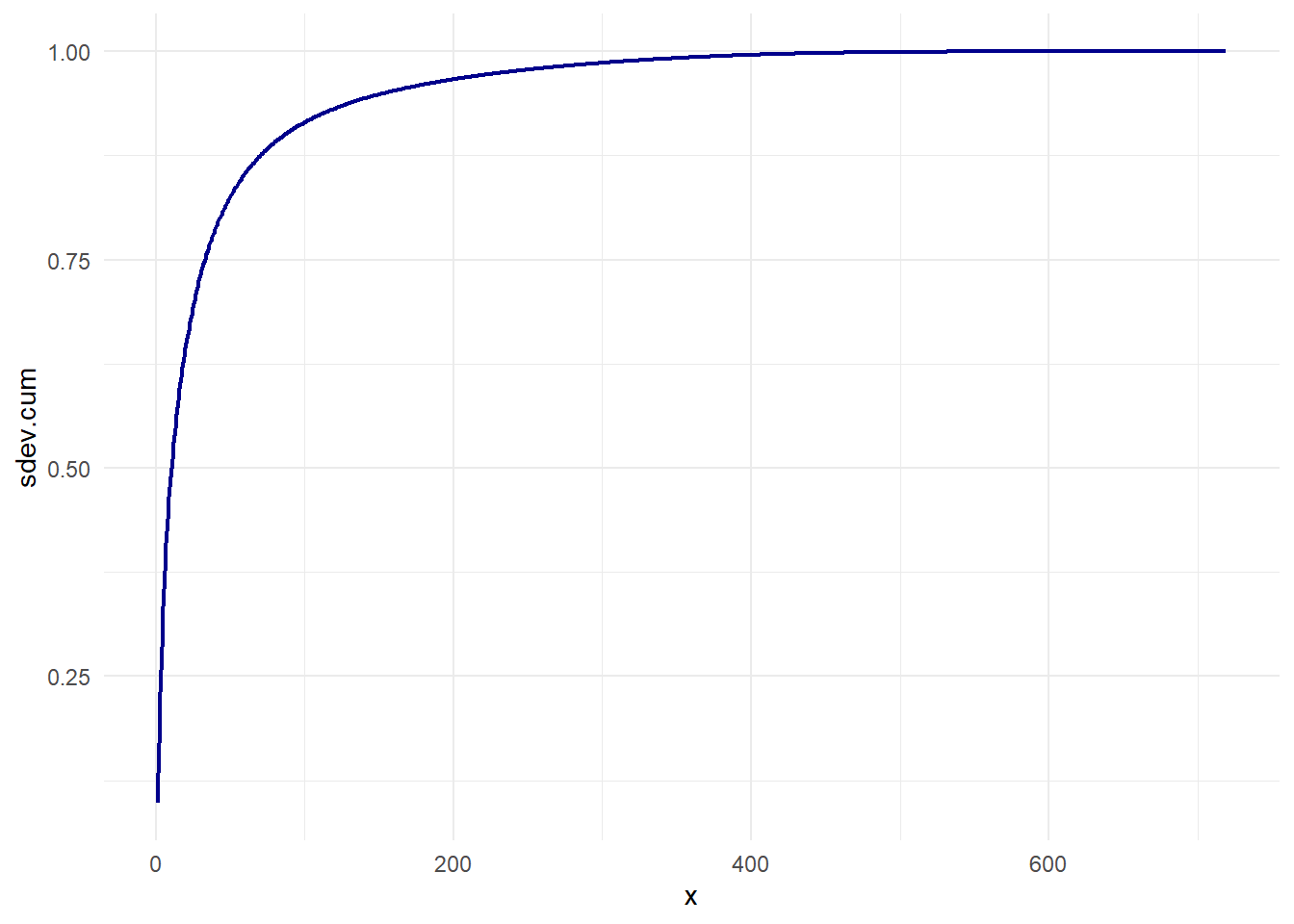
You can see in the chart above, we can get 90% of variance with only 80 of dimension from a universe of 719! This is a great information compression, almost 10:1!
Ploting cases in new PCA space
Lets see how the 200 first cases in the data set are distributed in the first two dimensions (15% the variation).
# lets see the distribution
pca.idx <- sample(1:mnist$train$n, 200)
cases <- tibble(
  label = as.factor(mnist$train$y[pca.idx]),
  x = tr.x[pca.idx,1],
  y = tr.x[pca.idx,2],
  z = tr.x[pca.idx,3]
)

# all cases
cases %>%
  ggplot(aes(x=x, y=y, color=label)) +
  geom_point(size=2, alpha=.5) +
  theme_minimal()
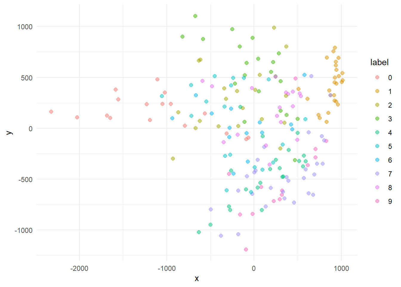
A little mess, but if we plot only the most distances centroids (0, 1 e 9) we already see a separable structures if only two dimensions.
# cases more "distant"
cases %>%
  filter(label %in% c("0", "1", "9")) %>%
  ggplot(aes(x=x, y=y, color=label)) +
  geom_point(size=2, alpha=.5) +
  theme_minimal()
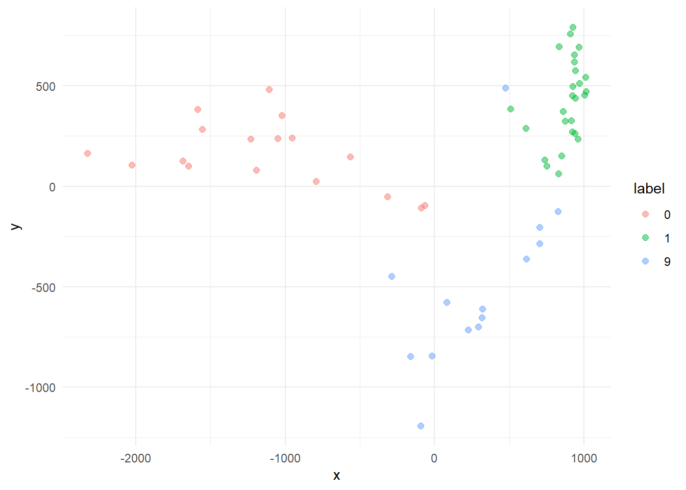
This sound promising. An kNN approach with higher dimension may do a decent job classifying the digits. Lets put another one, increasing the explained variation to 23%.
You can play around turning off the cases of some digits and rotating the chart. Can you see how the 0, 1 and 9 clusters are distributed in the space? And the 4 and 9 cases?
k-Nearest Neighbors
We saw that the PCA did a great job spreading the digits in the space, allow some separation, now let’s apply a kNN fit on this. We need to decide the number of dimension to be used (n) and the number of k-Nearest (k), to do this let’s make a cross validation search2.
# knn cross validation
part.idx <- sample(1:mnist$train$n, round(mnist$train$n/2))

# cross validation parameters
k <- seq(2,14, 2)
n <- seq(5,80,10)
cross.params <- crossing(k=k, n=n)

# fit a kNN Model for each cross validation pair, and calc the accuracy
result <- apply(X = cross.params,1, function(p, tr.idx = part.idx, x=tr.x, y=as.factor(mnist$train$y)){
  k_par <- as.integer(p[1])
  n_par <- as.integer(p[2])

  print(paste0("fitting: k=",k_par, " n=",n_par))

  y_hat <- knn(
    train = x[tr.idx,1:n_par],
    test=x[-tr.idx,1:n_par],
    cl=y[tr.idx],
    k=k_par
  )

  accuracy <- mean(y[-tr.idx]==y_hat)
  print(paste0("Accuracy: ", round(accuracy,4)))
  return(accuracy)

})

# build the CV results
cv.results <- bind_cols(cross.params, accuracy=result)
saveRDS(cv.results, "cv_result.rds") # to save time
str(cv.results)
The result is a data frame contain a pair of k and nand the accuracy that the kNN classifier get from this configuration
## tibble [56 x 3] (S3: tbl_df/tbl/data.frame)
##  $ k       : num [1:56] 2 2 2 2 2 2 2 2 4 4 ...
##  $ n       : num [1:56] 5 15 25 35 45 55 65 75 5 15 ...
##  $ accuracy: num [1:56] 0.681 0.943 0.962 0.966 0.966 ...
Let’s see the accuracy surface defined by k and n parameters.
# ploting the error "surface"
cv.results %>%
  wireframe(accuracy~n*k, .)
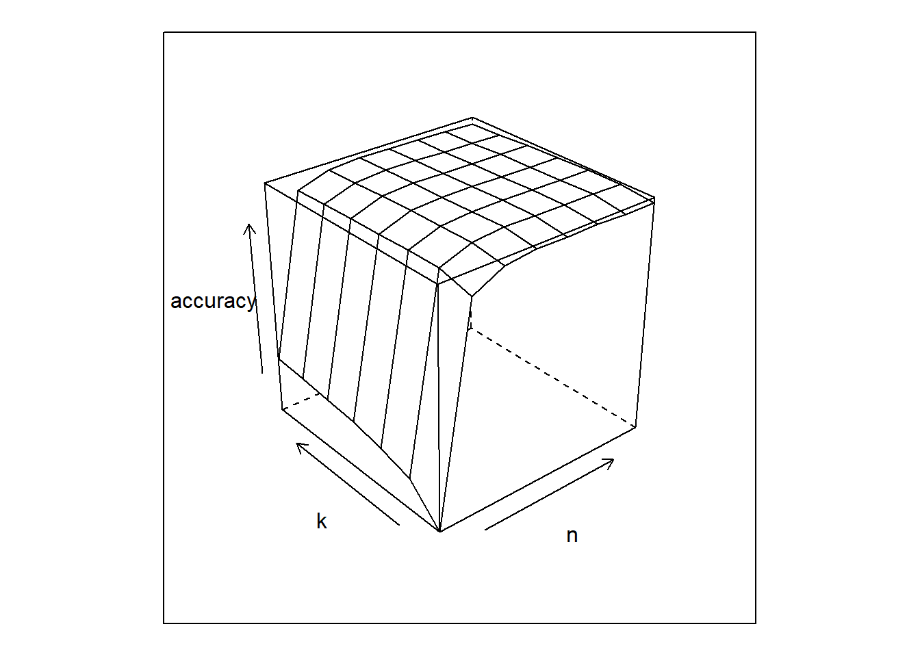
# which pair k and n are better ?
best <- cv.results[which(cv.results$accuracy==max(cv.results$accuracy)),]
The best result was k=4 and n=35, with an accuracy of 97%. Not so bad, comparing the 99% accuracy of LeNet ANN from the last post.
Conclusion
As we see, the data analysis on the MNIST data set allow us to realize that the digit recognition problem can be solved, with great accuracy, by a simple kNN model. Of course this is not a complete image recognition problem, an ANN would learn to separate the classes without our intervention.
But the analysis show that, in this case, we don’t need jump directly to an expensive ANN, and better than that, it indicates that not all 784 pixels are necessary do identify a digit and we can, for sure, use the kNN´s pre-classification as another input for the ANN, or fit independent ANNs for difficult cases like 4x9, showing another paths for model improvement.
References
This post was inspired by: